The Box–Muller transform turns two independent uniforms into two independent standard normals. Follow the radius-angle construction, its density proof and the zero-input trap.
Box–Muller transform
The Box–Muller transform converts two independent uniform random variables into two independent standard normal random variables. It supplies Gaussian shocks for Monte Carlo simulation, including the normal increments used to simulate diffusion models in option pricing. The transformation determines the output distribution; it does not create a good random-number source from a poor one.
Its useful surprise is that a pair of bell-shaped coordinates is easier to construct through a radius and an angle than through either coordinate's cumulative distribution function.
To obtain a normal variable with mean μ and standard deviation σ>0, use X=μ+σZ1. The second argument in N(μ,σ2) is the variance, so it is σ, rather than σ2, that multiplies the generated shock.
One fixed pair to check the arithmetic
Choose the stipulated demonstration inputs
u1=e−2,u2=81.
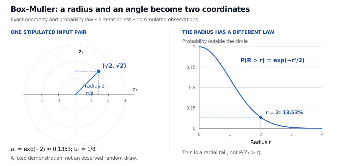
These are chosen numbers, not an observed random sample. They give
r=2,θ=4π,z1=z2=2≈1.414214.
The identity z12+z22=4 checks the radius. The equal positive coordinates check the first-quadrant angle. Two outputs being equal in this constructed example says nothing about dependence across random draws; independence is a property of the joint probability law.
Stipulated uniforms exp(−2) and 1/8 produce radius 2, angle pi/4 and coordinates (square root of 2, square root of 2). The theoretical radial tail at radius 2 is 13.53%, distinct from a one-coordinate normal tail.
Original exact construction and theoretical radial survival law, with no simulated observations. The point uses stipulated inputs; the curve describes the ideal random-input model.
Why the shared radius does not destroy independence
For r≥0, reversing the decreasing logarithmic transformation gives
P(R>r)=P(U1<e−r2/2)=e−r2/2.
Thus R has density fR(r)=re−r2/2 for r>0. The radius is not normally distributed. Its square has an exponential distribution with rate 1/2. The angle is uniform over a full turn and independent of the radius, because each comes from a different independent input.
The joint radius-angle density is therefore
fR,Θ(r,θ)=2πre−r2/2,r>0,0<θ<2π.
The polar-to-Cartesian Jacobian determinant has absolute value r. Dividing by this area factor yields the output density, apart from irrelevant sets of area zero:
That factorisation establishes two standard normal marginals and independence, rather than merely zero correlation. This is the geometric argument formalised in Vihola's Theorem 2.10.
If you instead hold R fixed at a positive value, the coordinates are constrained to one circle and are dependent. Box–Muller uses a random radius with exactly the law above; the fixed-radius conditional picture is a different distribution.
The boundary matters in actual software
The continuous model assigns probability zero to any exact endpoint. A finite-state generator may nevertheless return exactly zero. Substituting u1=0 makes lnu1 undefined. Use a documented positive-uniform convention or redraw a zero radial input; silently replacing zero with an arbitrary small constant changes the tail behaviour. Zero is harmless for the angle input. The deterministic boundary u1=1 gives radius zero.
Finite precision also means a generator cannot reproduce an unbounded continuous Gaussian law exactly: its smallest positive radial uniform bounds the attainable radius. That implementation limit does not mean the mathematical normal distribution has bounded support.
The Marsaglia polar method is a related rejection algorithm that avoids sine and cosine; it is a distinct procedure, not the trigonometric formula above. For a broader treatment, the Random Number Generation lesson covers both constructions and inversion. The full lesson requires membership; a public preview is available.
In production simulations, use a tested normal generator and record its seed and algorithm for reproducibility. Generating correct Gaussian shocks validates one ingredient of a model; it does not establish that market returns are Gaussian or that a discretised pricing model is accurate.