A bottom-up beta estimates a company's equity market beta from listed businesses with similar operating risks. It uses peers' stock returns to estimate the market exposure of the operations, then applies the financing of the company being valued. This gives an analyst a CAPM cost-of-equity input for a private business, a thinly traded company or a firm whose old share-price history reflects a different business mix.
Put the peers on a common footing
Suppose you are valuing a private packaging manufacturer. Start with listed peers whose demand moves with a similar set of customers and whose cost structures respond similarly when orders fall. A producer with fixed factory costs can have more market-sensitive earnings than a distributor selling the same product. Financial unlevering leaves that operating exposure in place, so business and cost structure both matter when screening peers. Damodaran, Estimating Risk Parameters, “Determinants of Betas”
Estimate each peer's equity beta from a regression of its stock excess returns on market excess returns, using a common market proxy, return frequency, currency and window where possible. Check that the window and leverage input represent the same business and financing regime. A recent recapitalisation can make today's debt ratio a poor match for a slope estimated mostly on older observations.
The Hamada equation provides the leverage conversion in this example. For peer , let and be market values of interest-bearing debt and equity, and the marginal corporate tax rate applicable to a usable interest deduction. Assume negligible debt beta and an interest tax shield with negligible market exposure valued at . Divide each equity beta by its own leverage multiplier to estimate the unlevered beta .
If non-operating cash is material, separate it before comparing operating betas. For an unlevered asset mix made up of operations and excess cash, with cash beta near zero, the mixed beta is the operating beta times the operating assets' share of that mix by value. Dividing by that share recovers the operating beta under the assumption. When the target beta needs to cover both operating and non-operating assets, put the target's cash back into the asset mix before applying its leverage. Keep the asset values and debt treatment on a consistent basis so the same cash is counted once. Damodaran, Ten Questions about Bottom-up Betas
The peer with the highest equity beta
Assume the following fictional peers have a 25% marginal corporate tax rate, negligible debt beta and no excess cash or preferred stock.
| Peer | Market debt-to-equity | Equity beta | Unlevered operating beta |
|---|---|---|---|
| A | 100% | 1.260 | 0.72 |
| B | 40% | 1.040 | 0.80 |
| C | 10% | 0.946 | 0.88 |
Peer A's equity beta is the highest, yet dividing by gives the lowest operating beta, . Equity holders are exposed to the operating result through a smaller equity base relative to its operating value. Giving these three adjusted estimates equal weight yields an operating beta of 0.80. Averaging can dampen estimation noise, but a common mismatch in demand exposure or a shared benchmark bias can survive the average. A sector shortcut pools the equity estimates first and un-levers with representative sector inputs. That shortcut and the firm-by-firm calculation can give different answers because each peer has its own divisor. Damodaran, Ten Questions about Bottom-up Betas
For a company with several businesses, estimate an operating beta for each business and weight them by each segment's share of the target's estimated operating value. That is a different weighting decision from pooling listed peers within a business. Segment enterprise values can be estimated from suitable peer multiples. Revenue weights implicitly give a dollar of revenue the same value across segments, which can misrepresent a high-margin or faster-growing business. Damodaran, Ten Questions about Bottom-up Betas, question 7
Apply the target's capital structure
The private manufacturer has a target market debt-to-equity ratio of 50%, a 25% marginal tax rate with usable deductions and negligible debt beta. It has only operating assets in this example. Under the same tax-shield assumption as the peers, multiplying by the target's leverage factor gives
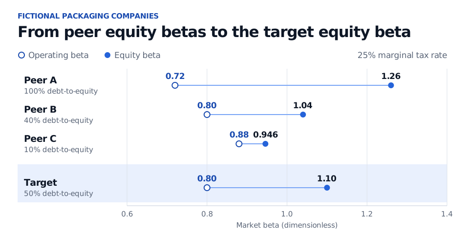
Peer A has the highest equity beta and the lowest operating beta. The target takes the peer mean of 0.80 and adds the effect of its own financing. All betas are dimensionless.
Use debt divided by equity for this adjustment. Use current market leverage when it represents the financing of the cash flows being valued. A forward-looking target may fit better if the valuation explicitly assumes a change in financing. Debt with a positive beta bears some of the firm's market risk. Changes in the risk or value of the tax shield also change the leverage adjustment. In those cases, revisit the model on both the peer and the target side. Hamada (1972), Section II and Damodaran, Estimating Risk Parameters, “Degree of Financial Leverage”
With a stipulated annual risk-free rate of 3% and an annual equity risk premium of 5%, the target's CAPM cost of equity is . The peer work supplies the beta. Step 3 of the SelfMadeQuant lesson derives how CAPM turns that exposure into a required return. The page offers a public preview and the full lesson requires membership. Derivation — CAPM from Portfolio Theory
Sources
- Aswath Damodaran, Ten Questions about Bottom-up Betas. Peer selection, consistent estimation, leverage and cash adjustments, and business-value weights.
- Aswath Damodaran, Estimating Risk Parameters. “Determinants of Betas” and “Bottom Up Betas,” PDF pages 22–30.
- Robert S. Hamada (1972), “The Effect of the Firm's Capital Structure on the Systematic Risk of Common Stocks”, The Journal of Finance 27(2), 435–452. Section II, especially equations (4)–(5), connects the equity and all-equity betas through the value of the financing tax shield.