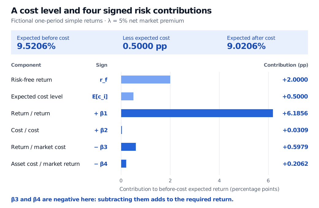
The liquidity-adjusted CAPM prices net return covariance and expected sale costs. A four-state example explains all four betas, their signs and the 9.5206% required return.
Acharya–Pedersen liquidity-adjusted CAPM
The Acharya–Pedersen liquidity-adjusted CAPM is an equilibrium asset-pricing model in which an asset's required expected return compensates for its expected trading cost and for the covariance of its after-cost return with the market's after-cost return. It extends the capital asset pricing model by making liquidity uncertain. For a quant, the useful distinction is between an asset that is expensive to sell on average and one that becomes expensive to sell in adverse market states.
Price the return that survives the sale
Use ri for the asset's one-period simple return before liquidity cost, and ci for its sale cost divided by the opening investment value. Thus a cost of 0.005 subtracts 0.5 percentage points from return; the after-cost return is ri−ci. Use the same convention for the market, rM−cM, and a matched risk-free simple return rf.
The original paper writes gross growth factors, such as 1+ri, rather than our simple returns. Subtracting one from both risky and risk-free growth factors preserves its pricing equation and every covariance. “Before cost” here does not mean a growth factor or a return before every conceivable fee and tax.
At time t, define
Dt=Vart(rM−cM)>0,λt=Et[rM−cM]−rf.
Acharya and Pedersen's central restriction is
Et[ri−ci]−rf=λtDtCovt(ri−ci,rM−cM).
All random returns and costs refer to the next period; the subscript t means conditional on today's information. Crucially, λt is the net market premium. Using the market's before-cost premium in its place changes the model. Acharya and Pedersen (2005), Proposition 1.
Why four betas have two minus signs
Expand the numerator using the bilinearity of covariance:
Call those four covariances, each divided by Dt, β1,β2,β3,β4 respectively. Then
Et[ri]=rf+Et[ci]+λt(β1+β2−β3−β4).
The table interprets these signs for positiveλt, holding the other terms fixed. A higher c always means worse liquidity, which prevents a common sign reversal.
Positive covariance supplies return when market trading is costly, reducing the required return.
−λtβ4
Asset cost with market return
Negative covariance means the asset becomes costly to sell when the market falls, raising the required return.
A minus sign in the formula does not mean that a channel always lowers required return. Subtracting a negative β3 or β4 raises it. Also, β1 uses net market variance in its denominator; it need not equal conventional market beta, whose denominator is Vart(rM).
Four states that make the signs visible
Consider an original fictional one-period scenario, with no annualisation. Independent shocks x and y each take values −1 and +1 with equal probability, giving four equiprobable states. Returns and costs below are decimal fractions of opening value:
Set rf=0.02. The asset mean μ will be chosen to satisfy the pricing restriction. Its value does not affect any covariance.
State (x,y)
Market before cost
Market cost
Asset cost
(−1,−1)
6%
1.1%
0.5%
(−1,+1)
6%
1.3%
0.7%
(+1,−1)
10%
0.7%
0.3%
(+1,+1)
10%
0.9%
0.5%
The down-market states have higher costs, and both costs are positive in every state. Market expected return after cost is 8%−1%=7%, so λ=7%−2%=5%.
Because rM−cM=0.07+0.022x−0.001y, independence gives
D=0.0222+0.0012=0.000485.
Compute population covariances by averaging across the four states, rather than applying a sample degrees-of-freedom correction. Their units are squared decimal return, and division by D makes each beta dimensionless:
Covariance numerator
Value
Beta
Cov(ri,rM)
0.000600
1.237113
Cov(ci,cM)
0.000003
0.006186
Cov(ri,cM)
−0.000058
−0.119588
Cov(ci,rM)
−0.000020
−0.041237
For example, the third numerator is 0.03(−0.002)+0.002(0.001)=−0.000058. Adding with the specified signs gives
or 9.5206%. Subtract the expected cost of 0.5 percentage points to obtain an expected after-cost return of 9.0206%. The expected excess return after cost is 7.0206 percentage points, rather than 9.5206%.
Fictional one-period return decomposition: risk-free return adds 2 percentage points, expected cost adds 0.5, and the four signed risk contributions add 6.1856, 0.0309, 0.5979 and 0.2062. Expected before-cost return is 9.5206% and after-cost return is 9.0206%.
Original fictional one-period example. Contributions are percentage points of before-cost expected return; negative third and fourth betas enter with minus signs and therefore make positive contributions.
This construction supplies internally consistent moments and a mean satisfying the equation. It does not solve for investors, asset supplies and clearing prices, so it is not a calibration or proof of a complete equilibrium. Nor is 9.5206% a guaranteed realised return: the four before-cost outcomes are approximately 6.3206%, 6.7206%, 12.3206% and 12.7206%.
Keep the level effect separate from risk
The E[ci] term reimburses an expected cost in the before-cost required return. The covariance terms price systematic exposure. To separate them algebraically, raise this example's ci by a constant 0.002 in every state. Its mean rises from 0.5% to 0.7%, while both covariances involving ci stay unchanged. Holding the market inputs and return covariances fixed, the equation's required before-cost return rises by 0.2 percentage points; its required after-cost return stays the same.
That is a controlled comparison of pricing inputs. An actual change in liquidity can also change prices, risk exposures and investor behaviour. Equating the whole adjustment with an average spread would discard those state-dependent risks.
The paper's tractable economy uses overlapping generations, one-period liquidation, risk-averse investors and exogenous trading costs. Its conditional result should not be replaced mechanically by a regression on raw historical liquidity levels: the empirical version treats liquidity innovations and requires additional assumptions. A fitted covariance is neither a causal effect of liquidity on return nor evidence that the equilibrium pricing restriction holds. Original model and empirical formulation, Sections 2–3.3.
For the portfolio-optimality argument behind ordinary beta pricing, Derivation — CAPM from Portfolio Theory, Steps 1–3, connects covariance to market clearing. Its preview is public; the full lesson requires membership. The liquidity extension changes the payoff being priced to the return remaining after sale costs.
Sources
Viral V. Acharya and Lasse Heje Pedersen (2005), “Asset pricing with liquidity risk”, Journal of Financial Economics77, 375–410. Section 2 explains the economy and sale costs; Section 3, Proposition 1, equations (7)–(8), gives the conditional pricing relation; Section 3.1 interprets the three liquidity risks; Section 3.3, equations (12)–(16), uses innovations in the empirical formulation. The four-state example and figure above are original illustrations, not empirical estimates from the paper.