Liquidity commonality measures how trading conditions move together. A five-date spread regression separates common liquidity movements from return covariance and priced risk.
Liquidity commonality
Liquidity commonality is the tendency for different assets' liquidity to move together through time, often with a market-wide or industry-wide component. For a quant managing a basket of trades, it means that holding many names need not diversify away the risk of trading conditions deteriorating together. Return diversification and liquidity diversification answer different questions.
Chordia, Roll and Subrahmanyam documented common movements in quoted spreads, effective spreads and quoted depth in NYSE stocks. Their 2000 paper studies the co-movement itself; it does not establish a universal liquidity risk premium. Commonality in liquidity, Sections 1–3.
Measure changes in liquidity, not returns
Choose a liquidity measure before estimating commonality. For example, express an asset's full proportional bid–ask spread in basis points:
Here a, b and m are the ask, bid and midpoint, with a positive midpoint and valid quotes. A higher S means a wider quoted spread and worse liquidity on this dimension. Define ΔSi,t=Si,t−Si,t−1, measured in basis points, and construct a market spread index excluding asset i. A simple descriptive regression is
ΔSi,t=αi+βiΔSM,−i,t+εi,t.
A positive slope says the stock's spread tends to widen when the other stocks' average spread widens, and narrow when it narrows. It does not say that either series causes the other. The slope measures sensitivity in the declared units; R2 measures the fraction of the stock spread-change variation captured by this particular fit.
A high average spread is a level of illiquidity. Commonality concerns its co-movement with other liquidity measures. A stock can be consistently expensive to trade without having a strong common component; a normally tight-spread stock can still widen alongside the market. The changes alone do not reveal the average spread.
Five fictional dates, one transparent fit
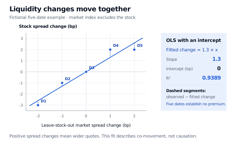
Suppose the following are matched daily changes in the proportional quoted spread. The market series is stipulated to exclude the stock; these are fictional observations, not market data.
Within this fit, a market widening of 1 bp corresponds to a fitted stock widening of 1.3 bp. That is a spread-change association, not a return of 1.3%, an expected trading profit or a forecast guaranteed to survive another sample.
The residual sum of squares is 1.10bp2 and the total centred sum of squares is 18bp2, so
R2=1−181.10=0.938888…≈93.89%.
Fictional stock and leave-stock-out market spread changes on five dates: market changes minus 2, minus 1, 0, 1 and 2 bp pair with stock changes minus 3, minus 1, 0, 2 and 2 bp. The fitted line has slope 1.3, intercept zero and R squared 0.9389; dashed segments show residuals.
Original fictional example. Both axes measure changes in proportional quoted spreads in basis points. The market index excludes the stock; the line is an OLS fit with an intercept. Its unusually high fit is chosen to make the arithmetic visible, not to represent typical empirical commonality.
The fit captures strong same-direction movement in these five observations. Five dates provide little evidence about stability, sampling uncertainty or stressed execution. In particular, no returns or expected-return observations appear in the table, so it cannot establish either return correlation or compensation for liquidity risk.
Keep three covariance questions separate
Let ri,rM denote asset and market returns, and let ci,cM denote comparable relative illiquidity costs, where larger costs mean worse liquidity. The following are different objects:
Covariance
Question
Cov(ri,rM)
Does the asset's return move with the market return?
Cov(ci,cM)
Does its trading cost rise when market trading costs rise?
Cov(ri,cM)
Does its return fall or rise when market trading becomes costly?
The middle row represents commonality in costs. The last row is a return exposure to market illiquidity. Neither is interchangeable with ordinary return covariance.
The Acharya–Pedersen liquidity-adjusted CAPM supplies an equilibrium model connecting expected costs and liquidity-related covariances to required returns. Under its assumptions, commonality in illiquidity is one priced channel; return sensitivity to market illiquidity and liquidity sensitivity to market returns are separate channels. A descriptive spread regression estimates none of those pricing restrictions by itself. Its basis-point changes in quoted spreads also cannot be substituted mechanically for the model's relative sale-cost variables. Acharya and Pedersen, Sections 2–3.1.
Before treating the coefficient as an exposure
The original commonality study used daily percentage changes in its liquidity measures, excluded the dependent stock from the market average, and considered lead–lag terms, market returns, volatility and industry effects. The example above instead uses basis-point differences in a proportional spread, so it illustrates the idea rather than reproducing that specification. Chordia, Roll and Subrahmanyam, Sections 2–3.1.
For an empirical application, the choices have concrete consequences:
Index composition: including the stock in its own market average builds a mechanical relationship into the fit. Excluding it avoids that direct overlap; it does not remove all dependence across stocks or identify a causal market shock.
Measure and sign: common widening of spreads and common shrinking of market depth can both indicate deterioration. A narrow spread alone says little about the quantity executable at that quote.
Timing and controls: use aligned observations and declared aggregation weights. Check whether market moves, sector composition, stale quotes or delayed adjustment account for the apparent relationship. A lead used for descriptive analysis would be unavailable to a real-time forecast.
Uncertainty and stability: assess residual dependence, coefficient uncertainty and behaviour across windows and market states. An in-sample fit supplies no guarantee that the next stressed exit has the same slope.
Commonality helps explain why several positions may become harder to trade at once. It is one component of market liquidity risk, whose practical consequences also depend on size, urgency and available depth. It does not, on its own, demonstrate contagion, a funding crisis or market collapse.
To build the underlying measurement correctly, Spread Measurement distinguishes quoted, effective and realised spreads, including their units and aggregation conventions. Linear Regression develops the slope, residuals and uncertainty behind the fit. Both have public previews; the full lessons require membership.