Variable elimination: Definition & Examples

Variable elimination is an exact inference algorithm that computes probabilities in a factorised model by multiplying relevant factors and summing out unwanted variables one at a time. In a quant risk model with hidden regimes and observable flags, it can calculate a flag probability without first storing the entire joint distribution.

Here, eliminating a variable means accounting for all its possible values, not deleting its influence or setting it to zero. The result is exact for the specified model in exact arithmetic; an implementation still has numerical precision limits.

Keep the calculation local

A factor is a function of a subset of the model's variables. For discrete variables, think of a table with one number per assignment. In a Bayesian network, the initial factors are its local probability tables. Intermediate factors need not sum to one.

To eliminate an unobserved variable $X$ :

Collect every current factor involving $X$ .
Multiply those factors, matching shared variable values.
Sum over $X$ and replace the collected factors with the resulting smaller factor.

Factors that do not involve

X

stay outside that sum. This is the distributive law applied to probability calculations, as explained in Berkeley CS188 §6.6. Retain the query variables until the end.

A hidden regime becomes a two-number message

Take the fictional binary chain $A\to B\to C$ : a regime, an intermediate risk flag and a final risk flag. The model assumes that $C$ depends on $A$ only through $B$ :

p(a,b,c)=p(a)p(b\mid a)p(c\mid b).

Let $p(A=0)=0.60$ and $p(A=1)=0.40$ , with conditional tables:

Condition	Probability of the next variable equalling one
$A=0$	$p(B=1\mid A=0)=0.20$
$A=1$	$p(B=1\mid A=1)=0.80$
$B=0$	$p(C=1\mid B=0)=0.10$
$B=1$	$p(C=1\mid B=1)=0.90$

All zero-state probabilities are complements. These inputs illustrate computation; they are not market estimates.

We want the marginal distribution of

C

. Eliminate

A

first:

\begin{aligned} f(b)&=\sum_{a=0}^{1}p(a)p(b\mid a),\\ f(0)&=0.60(0.80)+0.40(0.20)=0.56,\\ f(1)&=0.60(0.20)+0.40(0.80)=0.44. \end{aligned}

This factor happens to be the normalised distribution of $B$ . Multiply it by the remaining conditional table and eliminate $B$ :

p(C=1)=\sum_{b=0}^{1}f(b)p(C=1\mid b) =0.56(0.10)+0.44(0.90)=0.452.

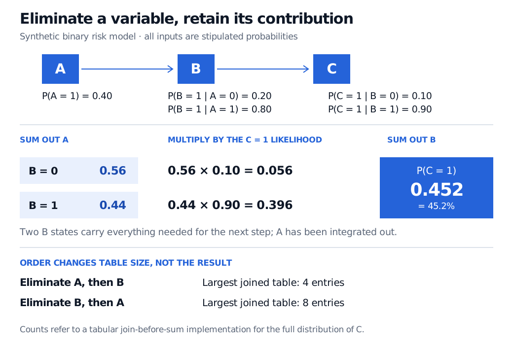
The four full-joint contributions with $C=1$ are $0.048$ , $0.108$ , $0.008$ and $0.288$ for $(A,B)=(0,0),(0,1),(1,0),(1,1)$ , respectively. Their sum is also $0.452$ . Elimination reuses the summed contributions rather than changing the probability.

Synthetic binary chain A to B to C. Summing out A gives B probabilities 0.56 and 0.44. Their contributions to C equalling one are 0.056 and 0.396, totalling 0.452. The largest joined table has four entries for order A then B, versus eight for B then A.

Original synthetic example. Summing out A preserves its contribution in a two-entry factor. The table-size comparison assumes explicit joins before summation and a query for the full distribution of C.

Evidence and normalisation

For a conditional probability query

p(Q\mid E=e)

, first restrict each affected factor to the observed values. Sum out variables that are neither query variables nor evidence. Multiplying the remaining factors produces an unnormalised function

g(q)

; normalise it:

p(q\mid e)=\frac{g(q)}{\sum_{q'}g(q')}.

The denominator must be positive. Evidence assigned zero probability by the model cannot yield a conditional distribution through this division. Poole and Mackworth §9.5.2 develops this procedure. Summing out an observed variable as though it were unobserved would discard the evidence.

Exact does not mean cheap

In the example, eliminating $A$ before $B$ requires joined tables over $(A,B)$ and $(B,C)$ , each with four entries. Eliminating $B$ first joins its two conditional factors into a table over $(A,B,C)$ with eight entries, before summing down to a four-entry factor over $(A,C)$ . Both orders give the same answer in exact arithmetic.

In larger networks, these differences can become exponential. A table over many variables contains an entry for every combination of their states. Elimination can connect formerly separate neighbours, creating large intermediate factors. An ordering's induced width describes this growth; treewidth is the minimum width over complete elimination orderings of the associated undirected graph. Choosing an order changes the computational burden, not the graph's minimum possible width. Poole and Mackworth §9.5.3 discusses this structural limit.

Heuristics such as min-fill help choose an order, but do not guarantee that inference will be affordable. Approximate inference may be necessary when intermediate factors are too large. The Stanford CS228 notes explain order selection and its effect on running time. The tabular procedure here covers finite discrete variables; continuous models require suitable integrals and factor representations.

For the model structure behind these calculations, Bayesian Networks and Markov Random Fields develops directed and undirected factorisations. Its preview is public; the full lesson requires membership.

Sources

UC Berkeley CS188, §6.6: Exact Inference in Bayes Nets: factor multiplication, summation and avoiding the full joint table.
Stanford CS228, Variable Elimination: factor operations, evidence and ordering heuristics.
Poole and Mackworth, Artificial Intelligence: Foundations of Computational Agents, 3rd ed., §§9.5.2–9.5.3: posterior normalisation, intermediate factor size and treewidth.

Keep the calculation local

A hidden regime becomes a two-number message

Evidence and normalisation

Exact does not mean cheap

Sources

Related terms

Bayesian network

Conditional probability

Joint distribution

Marginal distribution