Unspanned macro risk is macroeconomic variation that the current yield curve does not fully capture and that helps explain expected bond excess returns. A model can fit today's Treasury yields across maturities and still miss information about the expected reward for holding those bonds. That matters when using the curve to infer the path of future rates or to estimate a term premium. Joslin, Priebsch and Singleton, §§I–II
Same curve, different forecasts
Take two fictional states with identical model yield factors and therefore identical model yields at every maturity. A survey of expected inflation reads lower in state A than in state B. In each state the model forecasts the log return from buying a five-year Treasury zero-coupon bond and selling it a year later as a four-year bond. The excess return subtracts the log return on a one-year Treasury zero bought at the same time and held to maturity.
The model assigns a conditional expected excess log return of 0.5% in state A and 1.5% in state B. The gap is 1 percentage point, or 100 basis points. The two forecasts are stipulated. The survey comparison by itself cannot identify the effect of an inflation shock, and the realised excess return depends on the bond's future sale price.
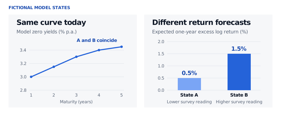
The fitted curve and the one-year benchmark are the same in both states. The model changes its forecast of the longer bond's return.
How prices and forecasts can come apart
In the Gaussian model of Joslin, Priebsch and Singleton, let be the vector of yield factors and the macro readings. The short rate depends only on . Under the risk-neutral measure used for pricing, the conditional distribution of future yield factors also depends only on . Together, these restrictions give the model yield at maturity the form
Holding fixed, has zero direct loading on model yields at every maturity. Macro readings can still be correlated with yield factors. Under the real-world measure , can change the forecast of future , and hence of future bond prices and excess returns. The difference between the two drifts changes the compensation for bearing yield-factor risk. An unchanged forward rate can then be consistent with a different expected future short rate and an offsetting change in its estimated forward premium. Joslin, Priebsch and Singleton, §II, equations (7)–(11), §V and Appendix B
The SelfMadeQuant lesson Martingale Measures and the Market Price of Risk derives how the difference between real-world and pricing drifts enters expected bond returns. The full lesson requires membership.
What the data can tell you
First ask how well today's yield factors reconstruct the macro reading. Project the reading on the factors and look at the residual. The residual measures what that particular yield-factor fit leaves unexplained. Next ask whether the residual helps predict future excess returns. In a linear regression with the same yield controls, adding the macro reading is equivalent to adding its residual. Joslin, Priebsch and Singleton used a Chicago Fed activity index and a Blue Chip survey of one-year inflation expectations. They found that these measures improved in-sample return fits relative to a three-factor yield benchmark. Joslin, Priebsch and Singleton, §I.A–B
A macro series can improve forecasts because it proxies for a yield factor that the analyst omitted or measured noisily. A richer yield-only benchmark could include further principal components or a forecast signal built from forward rates, such as a Cochrane–Piazzesi factor. Bauer and Rudebusch reproduced this pattern in simulated models where the macro information was spanned by the exact model curve. For a forecasting test, compare both forecasts on the same held-out dates. Use survey releases and macro data vintages that were actually available on each forecast date. Revised data can make the extra information look more useful than it was in real time. Predictive improvement is evidence about the chosen information set. Exact zero yield loadings are a separate structural hypothesis. Bauer and Rudebusch, §§2.2–2.3 and 5.1–5.2