How Stoll’s portfolio-cost theory explains inventory-sensitive dealer prices, with a signed risk-cost example and a careful distinction between quote shifts and spreads.
Stoll inventory model
The Stoll inventory model explains the compensation a dealer requires for accepting trades that change the risk of its portfolio. Its practical lesson for market making is directional: the same stock and trade size can be costly to buy and attractive to sell when the dealer is already long. Inventory affects willingness to trade, rather than just adding a fixed fee to every transaction.
Stoll's The Supply of Dealer Services in Securities Markets, published in 1978, develops this portfolio-cost approach. The original Wharton working paper, revised October 1977, starts with a desired investment portfolio and a separate trading account. Supplying immediacy moves the dealer away from its preferred position; compensation restores expected utility. The core assumes risk-free financing, terminal-wealth preferences, one transaction per trading interval and subsequent liquidation. Its short-period approximation includes trade size, dealer wealth and risk aversion, return variance and covariance with the existing trading account. Order and information costs are additional components. This is richer than a penalty on one stock's share count.
Put the trade on the dealer's side
A customer sale is a dealer purchase. If the dealer already owns 100 shares, accepting another 20 increases inventory to 120. A customer purchase instead takes 20 shares from the dealer, leaving 80. Reversing these directions reverses the economic interpretation.
To isolate that mechanism, consider an original reduced mean–variance illustration, not a restatement of all Stoll's assumptions. Let:
q be the dealer's signed inventory in shares, with a zero-share preferred position in this illustration;
v be the variance of the terminal price, measured in (USD/share)2, over one fixed holding horizon;
γ be a constant risk-aversion coefficient, measured per USD.
Hold expected price fixed, allow no intermediate hedging and exclude financing, processing and information costs. Assign the terminal inventory risk the monetary penalty
C(q)=2γvq2.
Since the variance of the inventory's terminal dollar value is q2v, this is the variance term of a mean–variance certainty equivalent. It is a utility-based valuation adjustment, not a bill paid in cash. In a real portfolio, covariance with other positions matters; a desired position need not be zero. If using excess inventory, define the target before calculating q.
Set γ=0.001USD−1 and v=4(USD/share)2. Thus the assumed terminal price standard deviation is USD 2 per share. These are fictional inputs, not an estimate for any security.
Dealer state or action
Inventory after trade
Holding-risk cost
Change from the starting cost
Starting position
100 shares
USD 20.00
—
Buys 20 from customer
120 shares
USD 28.80
+USD 8.80
Sells 20 to customer
80 shares
USD 12.80
−USD 7.20
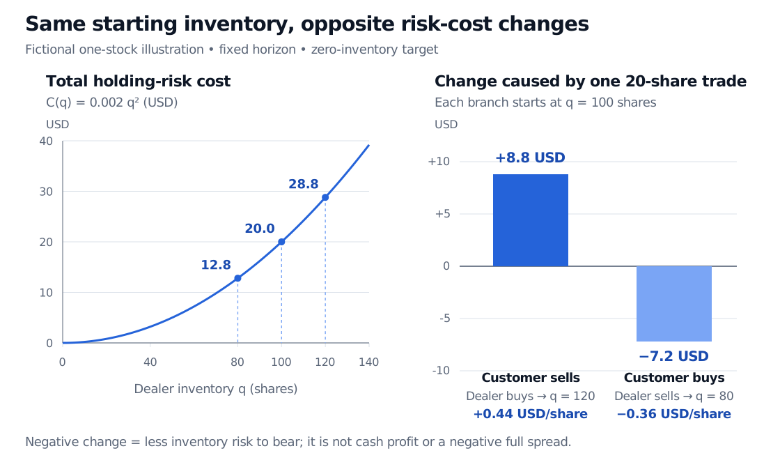
Both rows start from the same 100-share position; they are alternative trades, not a sequence. Buying adds 8.80/20=0.44 USD of risk cost per share. Selling changes risk cost by −7.20/20=−0.36 USD per share: the dealer benefits from reducing its exposure.
Fictional holding-risk cost curve: inventory 80, 100 and 120 shares costs USD 12.8, 20 and 28.8. From 100 shares, buying 20 adds USD 8.8; selling 20 reduces cost by USD 7.2.
Original reduced mean–variance illustration. The vertical quantities are utility-based risk costs in USD, not realised cash flows. Each trade branch starts from 100 shares.
The first line is a dealer purchase; the second is a dealer sale. The inventory term changes sign, while the trade-size term remains positive. A sale reduces this penalty when q>x/2. Selling far enough to create a large short position can increase it again. “Selling reduces risk” is therefore conditional on the starting position and trade size.
A negative increment is not a negative spread
The −USD 7.20 is a reduction in a modelled risk penalty. It is neither realised trading profit nor a full bid–ask spread.
For a concrete price interpretation, additionally assume zero carry and an expected terminal price m=50 USD per share. Let b and a denote risk-only indifference prices for buying or selling x=20 shares. Equating expected trading cash gain to the change in risk cost gives
At the bid, the dealer's expected gross gain of USD 0.44 per share compensates for extra risk. At the ask, it accepts an expected gross loss of USD 0.36 per share in exchange for reducing risk. This is indifference under the assumed objective, not a promise of a profitable fill.
The risk-only spread is still a−b=0.08 USD per share. With zero starting inventory, the same construction gives 49.96/50.04, also a USD 0.08 spread. The long position lowers both prices by USD 0.40, encouraging customers to buy from the dealer and discouraging further customer sales. Algebraically,
2a+b=m−γvq,a−b=γvx.
These equal-size, cost-covering formulas separate an inventory-driven quote shift from spread width. They are not an optimal market quote policy: processing costs, competition, financing, adverse selection and execution probabilities have been excluded. Stoll's own restricted cost-covering analysis also distinguishes inventory-sensitive prices from an inventory-independent spread; that result is conditional, not a universal empirical law. See §IV of the original working paper.
Where the dynamic model differs
The Ho–Stoll model of 1981 explicitly optimises a dealer's prices over time, with random transaction arrivals and return uncertainty. Its stochastic dynamic programme makes future trading opportunities part of today's quoting decision. The authors identify transaction uncertainty, an explicit multiperiod strategy and the demand side as distinguishing features. Stoll's earlier paper has a multiperiod extension too; the distinction is not simply “1978 has one date, 1981 has many.” Ho and Stoll's original working-paper introduction explains the difference.
For measurement rather than theory, Spread Measurement works through quoted, effective and realised spreads, including the factor of two between a one-way concession and full-spread units. The preview is public; the full lesson requires membership. That distinction helps prevent an inventory-risk calculation from being reported as observed spread revenue.
Sources
Hans R. Stoll, The Supply of Dealer Services in Securities Markets, Working Paper No. 2-78, revised October 1977. Original manuscript used here: §§I–V, especially §III equations (14)–(15), §IV equation (16), and the opening of §VII. The quadratic share-inventory example and figure above are original reductions, not the paper's full portfolio specification.
Hans R. Stoll (1978), The Supply of Dealer Services in Securities Markets, Journal of Finance 33(4), 1133–1151. Publisher record checked for final publication details; the model text read was the dated working-paper version linked above.
Thomas Ho and Hans R. Stoll (1981), Optimal dealer pricing under transactions and return uncertainty, Journal of Financial Economics 9(1), 47–73. Publisher abstract checked for stochastic arrivals, return uncertainty and dynamic programming; used to distinguish the dynamic model, not as the source of the reduced calculation.