A dynamic dealer model in which quote-dependent trading arrivals and risky portfolio returns determine inventory-sensitive bid and ask prices.
Ho–Stoll model
The Ho–Stoll model is a dynamic dealer quotation model: bid and ask prices balance trading revenue against portfolio risk. Its central lesson is that inventory can shift both quotes, rather than merely widen their spread.
The original dealer problem
In Ho and Stoll (1981), §§2–3, one dealer passively trades one stock in fixed quantities Q. Customer buys and sells arrive through independent, quote-dependent Poisson processes. The quotes are p+a and p−b; symmetric linear demand later sets λa=α−βa and λb=α−βb, within nonnegative-rate domains.
With dNa,dNb counting dealer sales and purchases, their account dynamics are
F is cash, I inventory value, and Y base portfolio wealth. Wiener shocks have variances σI2dt,σY2dt and covariance σIYdt. Constant p is an accounting convention: uncertain returns appear as continuous dividends. Shorting and borrowing are allowed.
The dynamic programme chooses feedback fees a,b from state (t,F,I,Y):
Terminal liquidation is costless. The paper approximates fee effects and expands the value function in time; its later mean–variance calculation uses quadratic utility. It is not a CARA-normal closed-form quote rule.Original paper, §§2–6.
Isolate the inventory mechanism
A smaller calculation makes the intuition visible without pretending to solve that dynamic programme. This is an original, fictional one-period CARA-normal illustration: no future trading arrivals, no other risky assets, no financing costs and no execution optimisation. Shares are held to the horizon.
Let terminal price be ST∼N(m,v), measured in USD/share, and let cash plus stock wealth be X+qST, with q measured in shares. Use exponential utility
U(W)=−e−γW,γ>0.
Here γ is constant absolute risk aversion, in inverse dollars. Normality makes the certainty equivalent exactly
C(X,q)=X+qm−2γq2v.
To see why, the normal exponential moment gives expected utility −exp{−γ(X+qm)+γ2q2v/2}. Equating this to −e−γC yields the expression above. This is an expected-utility comparison, not a no-arbitrage price shared by every trader.
The marginal value of an extra share is
r(q)=∂q∂C=m−γqv.
A long dealer values another share less because it adds to inventory risk. A short dealer has the opposite exposure. This calculation's zero-inventory reference relies on the absence of other risky positions; correlated portfolio exposures would change it.
A marginal centre is not a whole-share bid or ask
For a transaction of h>0 shares, define the reservation bidBh as the highest price per share the dealer will pay while remaining indifferent:
C(X−hBh,q+h)=C(X,q).
Define the reservation askAh as the lowest acceptable sale price:
C(X+hAh,q−h)=C(X,q).
Subtract the certainty equivalents and divide by h:
The midpoint equals the marginal centre here because the inventory penalty is quadratic. Neither whole-unit price equals that centre. Both approach it as h→0.
Take m=100, v=4, γ=0.001 per dollar, q=10 shares and h=1 share. The variance is 4 squared USD/share units, so the terminal price standard deviation is 2 USD/share. The calculation gives
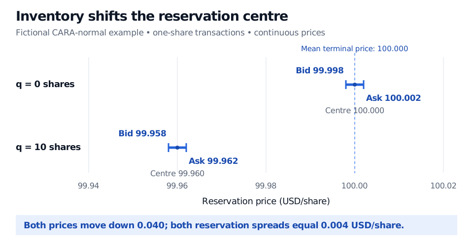
All three prices are USD/share. Buying at 99.958 or selling at 99.962 leaves the dealer's certainty equivalent unchanged. At q=0, the bid and ask are 99.998 and 100.002. Inventory therefore moves both prices down 0.040 USD/share, while the whole-share reservation spread stays 0.004 USD/share. Long inventory need not make the spread wider.
Fictional one-period CARA-normal example. At zero shares the reservation bid is 99.998 and ask 100.002. At ten shares they are 99.958 and 99.962. Both centres differ by 0.040 USD per share; both reservation spreads equal 0.004 USD per share.
Original reduced illustration: inventory shifts the reservation centre while the whole-unit reservation spread stays fixed. These are indifference prices, not dynamically optimal Ho–Stoll quotes.
Indifference is not an execution strategy
Posting these reservation prices would make each stipulated trade just acceptable under the reduced assumptions. It says nothing about how often a customer accepts them. A profitable quoting policy must also weigh the gains from changing price against the resulting change in arrival rates and future inventory. That requires a continuation value, not just the current holding's certainty equivalent.
Do not label the numerical pair above “the optimal Ho–Stoll quotes” or an Avellaneda–Stoikov formula. Similar-looking inventory shifts do not make different objectives, return processes and demand specifications interchangeable. Nor is a reservation spread a realised trading profit: actual fills, subsequent prices and costs matter. The example also permits sub-cent prices; an executable policy must respect its venue's tick and order constraints.
Spread Measurement develops the difference between quoted, effective and realised spreads, and why a favourable initial fill can lose against a later midpoint. Its preview is public; the full lesson requires membership.
Sources
Ho, T. and Stoll, H. R. (1981), Optimal dealer pricing under transactions and return uncertainty, Journal of Financial Economics 9(1), 47–73. Original journal version, especially §2, account dynamics and terminal liquidation; §3, dynamic programming; §§4–6, approximations and pricing strategy. The CARA-normal example above is a separate derivation, not a reproduction of the paper's numerical illustration.