Signal-to-noise ratio compares a defined signal with a defined noise component. Distinguish power, variance and RMS conventions, decibels and financial predictability.
Signal-to-noise ratio
Signal-to-noise ratio (SNR) compares the strength of a specified signal with that of a specified noise component. Under the power convention, it is signal power divided by noise power. For a quant, its usefulness starts with the definition of the components: a price-measurement problem and a return-forecasting problem can call entirely different quantities “signal”.
State what the ratio measures
Write an additive model X=S+N: X is observed, S is the target component and N is the disturbance relative to that target. For real random variables with finite second moments, define mean-square powers by
PS=E[S2],PN=E[N2],SNRpower=PNPS,PN>0.
Here “power” is a statistical mean square, in squared units of the quantity being measured. It need not be physical power in watts. Define both components over the same measurement horizon and under the same filtering or frequency-band convention.
A root-mean-square (RMS) amplitude is AS=PS, and similarly for noise. Therefore
SNRdB=10log10(PNPS)=20log10(ANAS).
The factor is 10 for power, 20 for RMS amplitude. These are the conventions shown in MIT's noise lecture; Rice's laboratory notes explain the mean-square/RMS relationship. Positive finite powers are needed for a finite dB value. Equal powers give 0 dB; a negative dB value means noise power exceeds signal power.
Power equals variance only for a mean-zero component, because
E[S2]=Var(S)+E[S]2.
With nonzero means, say whether the level itself is the signal or whether components have been centred. A centred variance ratio and an uncentred power ratio generally differ. RMS amplitude then also differs from standard deviation.
Four times the power means twice the RMS amplitude
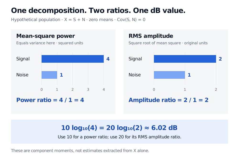
Take a hypothetical population with E[S]=E[N]=0, Var(S)=4 and Var(N)=1 in squared measurement units. Assume zero covariance between the components. One exact construction gives S values −2 and +2, and independently gives N values −1 and +1, with each sign equally likely.
The power SNR is 4/1=4. The RMS amplitude ratio is 2/1=2. Their common dB representation is
10log10(4)=20log10(2)≈6.0206 dB.
Hypothetical mean-zero uncorrelated components: signal power 4 and noise power 1 in squared units give SNR 4; signal RMS 2 and noise RMS 1 in original units give amplitude ratio 2. Both yield 6.02 dB.
Original comparison of stipulated population moments. Each panel uses its own labelled scale: power is in squared units, while RMS amplitude is in original units. The ratio changes when taking square roots; its correctly calculated dB value does not.
Uncorrelatedness matters when adding component variances:
Var(X)=Var(S)+Var(N)+2Cov(S,N)=5.
The signal accounts for 4/5=80% of observed variance under this stipulated decomposition. That fraction is not the SNR: the SNR compares signal with noise, rather than with the total. Similarly, observed power divided by noise power is 5/1=5, a signal-plus-noise to noise ratio. If signal and noise are correlated, the covariance term prevents the same additive allocation; independence is sufficient for zero covariance but is stronger than necessary.
A financial signal need not be a trading forecast
For estimating an efficient price, the desired signal can be an unobserved efficient log-price, while noise represents transaction-price disturbances. Aït-Sahalia, Mykland and Zhang's model uses this decomposition with mean-zero independent observation noise. Bid–ask effects and price discreteness motivate the disturbance. The paper also discusses relaxing independence. This is a measurement model: recovering price variation does not automatically predict the direction of the next return. Its components and sampling horizon must be specified before reporting an SNR.
Nor does the observed series alone identify its latent components. Even a population observation distributed normally with mean zero and variance 5 could be the sum of independent normal components with variances 4 and 1, or with variances 1 and 4. These have the same observed distribution but power SNRs of 4 and one quarter. Identification needs additional information or restrictions, such as repeated measurements, a noise model or justified dynamic structure. A smooth fitted curve is not automatically the true signal.
Finance also uses “signal-to-noise” informally for a mean relative to uncertainty. Always inspect the formula:
A Sharpe ratio divides mean excess return by its standard deviation; it is signed and is not this power ratio.
A mean's test statistic divides its estimated distance from a null value by an estimated standard error; its scale depends on the sample and dependence assumptions.
Forecast predictability depends on the information available before the outcome. A high power SNR for a component visible only afterwards does not establish usable predictive skill or profitable trading after costs.