Semipartial correlation: Definition & Examples

Semipartial correlation is the correlation between one variable and the linear-regression residual of another after selected controls have been removed from that second variable. In a factor study, it can measure how much an additional factor contributes to explaining a return series once existing factors are already included. Only one side is residualised; that choice matters.

For a response $Y$ , candidate predictor $X$ and control $Z$ , write

X_{\perp Z}=X-a-bZ, \qquad s_{Y(X\mid Z)}=\operatorname{Corr}(Y,X_{\perp Z}).

Here

a+bZ

is the population least-squares linear projection of

X

on an intercept and

Z

. In a sample, use the corresponding ordinary least squares fit and its residuals. The notation puts parentheses around the side being adjusted. The response

Y

retains its original variance. This is also called a part correlation.

A candidate factor beyond the market

Consider a fictional population of monthly observations: $Y$ is a fund's excess return, $X$ a candidate factor return and $Z$ the market excess return. Stipulate the jointly valid population correlations

r_{YX}=0.60,\qquad r_{YZ}=0.50,\qquad r_{XZ}=0.40.

These are illustrative population inputs, not estimates from a market dataset. For one control, the residual formula gives

s_{Y(X\mid Z)} =\frac{r_{YX}-r_{YZ}r_{XZ}}{\sqrt{1-r_{XZ}^2}} =\frac{0.60-0.50(0.40)}{\sqrt{0.84}} \approx 0.4364.

The numerator removes the covariance associated with the linear projection on $Z$ . The denominator accounts for the smaller variance of the residualised $X$ . There is no corresponding shrinkage of $Y$ in this denominator.

By contrast, partial correlation residualises both $X$ and $Y$ on the same control. Its value is

p_{YX\mid Z} =\frac{0.60-0.50(0.40)}{\sqrt{0.84}\sqrt{0.75}} \approx 0.5040.

The larger number uses a different reference variance. It does not represent a second improvement in the fit.

The square is an increment in R-squared

For nested linear projections of $Y$ with an intercept, adding the single predictor $X$ to controls $Z$ gives

s_{Y(X\mid Z)}^2 =R^2_{Y\sim Z+X}-R^2_{Y\sim Z}.

The identity also holds for unweighted sample OLS when both models use exactly the same observations and the usual centred R-squared. It extends to a vector of controls by residualising

X

on all of them together. The residualised predictor must have nonzero variance.

Why does this work? The component $X_{\perp Z}$ is orthogonal to the existing predictor space. Its extra fitted component therefore contributes an additional, orthogonal piece of explained variation. Dividing that increment by the total variation in $Y$ gives its squared correlation with $Y$ .

In the fictional population:

Quantity	Value	Denominator
Market-only $R^2$	$0.2500$	Total $Y$ variance
Full $R^2$ with market and candidate factor	$0.440476$	Total $Y$ variance
Squared semipartial correlation	$0.190476$	Total $Y$ variance
Squared partial correlation	$0.253968$	$Y$ variance remaining after market

The candidate factor adds 19.05 percentage points to explained variance. It explains 25.40% of the variance left after the market, since

0.190476/(1-0.25)=0.253968

. These are two descriptions of the same increment.

Fictional population: market Z explains 25% of Y variance, adding X explains 19.05% more and 55.95% remains unexplained. Squared semipartial correlation is 19.05 divided by 100; squared partial correlation is 19.05 divided by the remaining 75.

Original fictional population example. Both bars use original Y variance as their horizontal scale; the lower bracket marks the smaller denominator used by squared partial correlation. Values shown in the graphic are rounded.

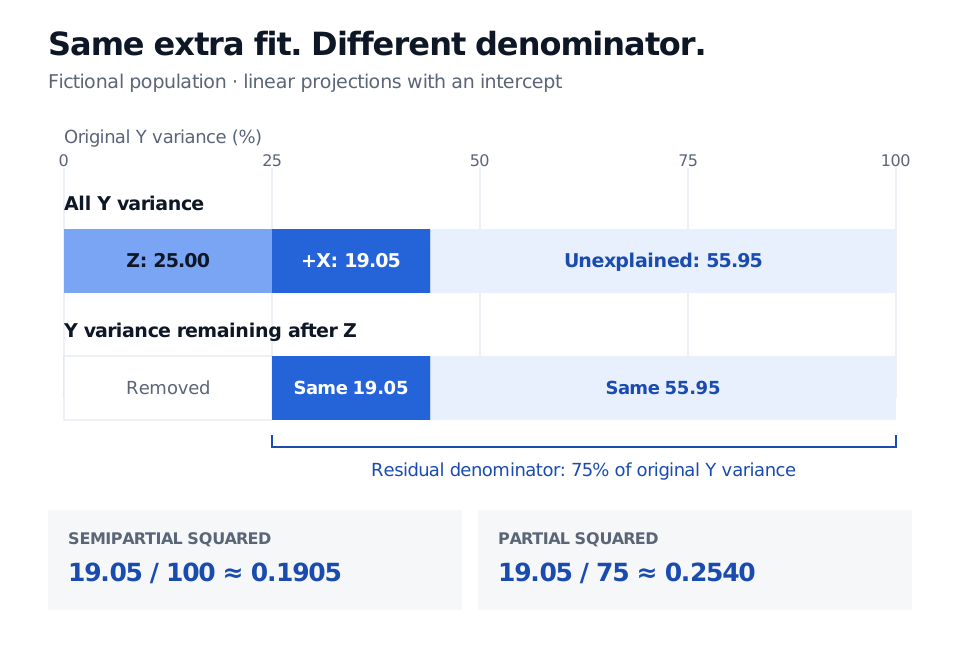
Read the direction and the model

Residualising $Y$ instead gives $\operatorname{Corr}(X,Y_{\perp Z})\approx0.4619$ in this example, rather than $0.4364$ . State which variable was adjusted. Squaring also discards the sign: reversing the sign of the candidate factor reverses its semipartial correlation while leaving the increment in $R^2$ unchanged.

“Unique contribution” means incremental linear fit relative to the specified controls. Changing those controls changes the quantity. Last-added contributions from several correlated predictors need not sum to the full model's

R^2

; a sequential decomposition uses a different conditioning set at each step.

A zero semipartial correlation does not exclude nonlinear dependence. Nor does residualising on a market factor identify a causal effect or establish performance on future observations. In a sample, the raw in-sample $R^2$ increment cannot be negative, even for a useless extra predictor. Use separate inference and dated validation to assess sampling noise and forecasting usefulness.

Correlations require finite, nonzero variances; the residualised side must also have nonzero variance. Arbitrarily chosen pairwise correlations may fail to form a positive semidefinite correlation matrix. Exact linear redundancy makes the residual correlation undefined, rather than zero.

For the nested-model geometry and tests behind this interpretation, Multiple Linear Regression develops full and reduced fits and the partial F-test (public preview; full lesson requires membership).

Sources

Philip B. Ender, UCLA: Partial and Semipartial Correlation — definition through removing controls from predictors only.
MRC Cognition and Brain Sciences Unit: Computing the semi-partial coefficient for a predictor — signed square root of the difference in model R-squared values.
Algina, Keselman and Penfield (2008): Note on a Confidence Interval for the Squared Semipartial Correlation Coefficient — the original paper's abstract defines the squared coefficient as incremental explained variance; the full paper is access restricted.

A candidate factor beyond the market

The square is an increment in R-squared

Read the direction and the model

Sources

Related terms

Coefficient of determination

Correlation

Ordinary least squares

Residual