Reallocating equity exposure among sectors using dated signals. Follow a 70/30 tilt, its benchmark-relative gain or loss, turnover, costs and changing risks.
Sector rotation
Sector rotation is the deliberate reallocation of equity exposure among sectors or industries as their expected relative returns change. A portfolio might move capital between technology, energy and utilities in response to a macroeconomic forecast, a commodity-price shock or a price-based signal. For a quant, the central question is whether information available before the trade helps choose sector weights that improve results after costs and risk.
The sector is the unit of allocation. Changing the equity–bond mix is tactical asset allocation; changing which companies to own inside an unchanged sector allocation is stock selection. Sector rotation can accompany both. A rule that favours recent industry winners is an industry momentum implementation of rotation, rather than a necessary feature of every rotation strategy.
First specify what can rotate
“Buy cyclicals before a recovery” leaves most of a strategy undefined. Which stocks or funds qualify as cyclicals? What information identifies a recovery, when was it released, and at what price could the portfolio trade? A reproducible rule needs an eligible universe, a classification history, signal timestamps, a weighting rule and a rebalance schedule.
Classification itself matters. The October 2026 GICS methodology distinguishes sectors, industry groups, industries and sub-industries; companies are assigned according to their principal business activities. Its maintenance and chronology sections describe classification reviews and structural changes. A historical test therefore needs the groups and constituents applicable at the time. Applying today's sector map retrospectively can change what the strategy appears to have held.
The traded instrument also matters: a sector index is a return benchmark, while a fund tracking it has its own fees, spreads, holdings and tracking differences. Owning energy equities is not equivalent to holding oil futures. A higher oil price can affect producers, refiners and energy users differently, and the price move may already be reflected in their shares.
A dated trade, then two possible outcomes
Consider a fictional, long-only universe containing only two eligible sector funds: A represents technology and B represents utilities. Both are already investable, denominated in the same currency and available throughout the example. They are teaching instruments, not named products.
The rule is declared in advance: after each month-end close, compare the two funds' completed one-month simple total returns; at the next month's opening execution, allocate 70% to the higher-return fund and 30% to the other. A tie gives 50/50. Hold until the next scheduled rebalance. The rule and weights are illustrative assumptions, with no claim that this lookback or allocation is effective.
After the 30 September 2026 close, the observed returns are A +3% and B +1%. The signal therefore selects A. At the 1 October opening execution, weights become 70/30. The comparison benchmark portfolio starts the same holding interval at 50/50. Both hold without interim trading through the 30 October close. Assume exact fills at the stipulated starting weights, reinvested distributions, no external flows, no leverage and no currency effect. The subsequent returns below run from that opening execution to the ending close; they are not the September signal returns.
Outcome revealed after execution
A return
B return
Rotation return
Benchmark return
Active return
A subsequently leads
+4%
−2%
+2.2%
+1.0%
+1.2 percentage points
B subsequently leads
−2%
+4%
−0.2%
+1.0%
−1.2 percentage points
For beginning weights ws, benchmark weights bs and holding-period sector returns Rs, the gross arithmetic active return is
RP−RB=s∑(ws−bs)Rs.
Here the active weights are +0.20 in A and −0.20 in B. Consequently,
RP−RB=0.20(RA−RB).
In the first outcome, 0.7(0.04)+0.3(−0.02)=0.022, while the benchmark earns 0.5(0.04)+0.5(−0.02)=0.01. Reversing the realised sector returns reverses the active contribution. The signal and the weights stay fixed in both rows. Selecting the winning row after observing October would introduce look-ahead bias.
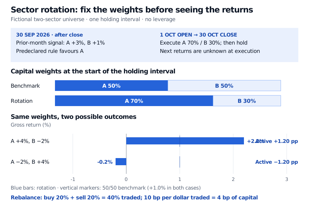
A fictional signal observed after 30 September selects A at 70% and B at 30% for the October holding interval, versus a 50/50 benchmark. A +4%, B −2% yields rotation +2.2% and active +1.2 percentage points; reversing the returns yields rotation −0.2% and active −1.2 percentage points. Forty percent traded at 10 basis points per dollar costs 4 basis points of capital.
Figure: Original fictional allocation and outcome comparison. Weights are fixed before the holding-period returns; bars show gross portfolio returns and vertical markers show the benchmark. The cost line refers only to the initial rebalance.
The trade has a price
Suppose that immediately before execution the portfolio is also 50/50. Reaching 70/30 requires buying 20% of capital in A and selling 20% in B. Total absolute traded weight is 40%; the half-sum convention for one-way portfolio turnover reports 20%. These are different denominators for the same trades.
Stipulate a cost of 10 basis points per dollar bought or sold. The rebalance costs 0.001×0.40=0.0004 of starting capital, or 4 basis points. For transparent accounting, this toy ledger records that cost as a fixed liability paid at the end of the holding interval, with no financing charge. It leaves the gross 70/30 holdings unchanged. An upfront deduction would require adjusting invested notionals and would give a slightly different result.
On starting capital of USD 1 million, the favourable outcome produces USD 22,000 gross profit, less USD 400 costs: USD 21,600 net profit. The unchanged benchmark earns USD 10,000 with no trading cost in this example. Net active return is 1.16 percentage points, or USD 11,600. In the reversal, the same cost makes net active return −1.24 percentage points. There is no terminal liquidation or later rebalance cost in either figure.
A full backtest must charge subsequent trades too, using the weights that have drifted with prices immediately before each rebalance. Commissions alone can miss spreads, market impact, taxes and fund expenses; the cost model must also avoid counting costs already included in a fund's reported returns twice.
Why a business-cycle diagram is not a trading rule
A cyclical sector may be sensitive to economic activity, but that does not establish when its shares will outperform a defensive sector. Prices respond to expectations, surprises, valuations and discount rates as well as realised business conditions. A sector can have growing earnings and still underperform if investors had expected stronger growth.
For a macro-conditioned rule, store the actual release time and the data vintage available then. A cycle label constructed afterwards by splitting a completed expansion into early, middle and late thirds cannot identify those thirds in real time without knowing the future ending date. That is a different experiment from trading on contemporaneous indicators.
Molchanov and Stangl's original study, first published in 2023, directly tests conventional business-cycle sector rotation. It finds limited support for systematic outperformance, with results weakened by costs and cycle mistiming even when the baseline grants perfect cycle timing. The authors explicitly limit the conclusion: it does not show that every strategy using sector or industry information is impossible. It challenges the automatic mapping from cycle stage to winning sector.
Finally, rotation changes risk. A portfolio can remain fully invested in equities while increasing market beta, interest-rate sensitivity, commodity exposure or concentration. Positive benchmark-relative return over one interval does not identify alpha. Evaluation needs a declared benchmark, several market environments, realistic implementation and performance adjusted for the exposures the rule actually took.
For the distinction between deliberate sector allocation and stock-selection signals constrained to match benchmark sector weights, see Portfolio Constraints (public preview; full lesson requires membership).