Rectangle rule: Definition & Examples

The rectangle rule approximates a definite integral by replacing a changing function with a constant height on each small interval, then adding height times width. The height can come from the left endpoint, right endpoint or midpoint. State that choice: “rectangle rule” alone does not identify a unique numerical answer.

In finance, a rectangle can represent a cash-flow rate in USD/year multiplied by a time step in years, producing a cash amount in USD. For an expected payoff, the height is instead the payoff multiplied by its probability density. Sampling the payoff alone would omit the probabilities.

Which height are you using?

For $a<b$ , split $[a,b]$ into $n$ equal panels with

h=\frac{b-a}{n},\qquad x_i=a+ih,\qquad i=0,\ldots,n.

The three choices give

\begin{aligned} L_n&=h\sum_{i=0}^{n-1}f(x_i),\\ R_n&=h\sum_{i=1}^{n}f(x_i),\\ M_n&=h\sum_{i=0}^{n-1}f\left(x_i+\frac h2\right). \end{aligned}

Each uses one sampled value per panel. On an irregular grid, replace $h$ by each panel's own width; multiplying every height by an average spacing generally gives a different calculation. These finite approximations are Riemann sums. Their limiting value, when the mesh shrinks and the function is Riemann integrable, is the integral.

MIT's explanation of integration rules distinguishes the three height choices. The midpoint rule is a rectangle rule even though the curve need not stay above or below each rectangle.

Three heights for the same curve

Take the synthetic, dimensionless function $f(x)=x^2$ on $[0,1]$ , with exact integral $I=1/3$ . Equivalently, this is the second moment of a uniform random variable on $[0,1]$ , where the density is one. This is a numerical benchmark, not a model calibrated to market returns.

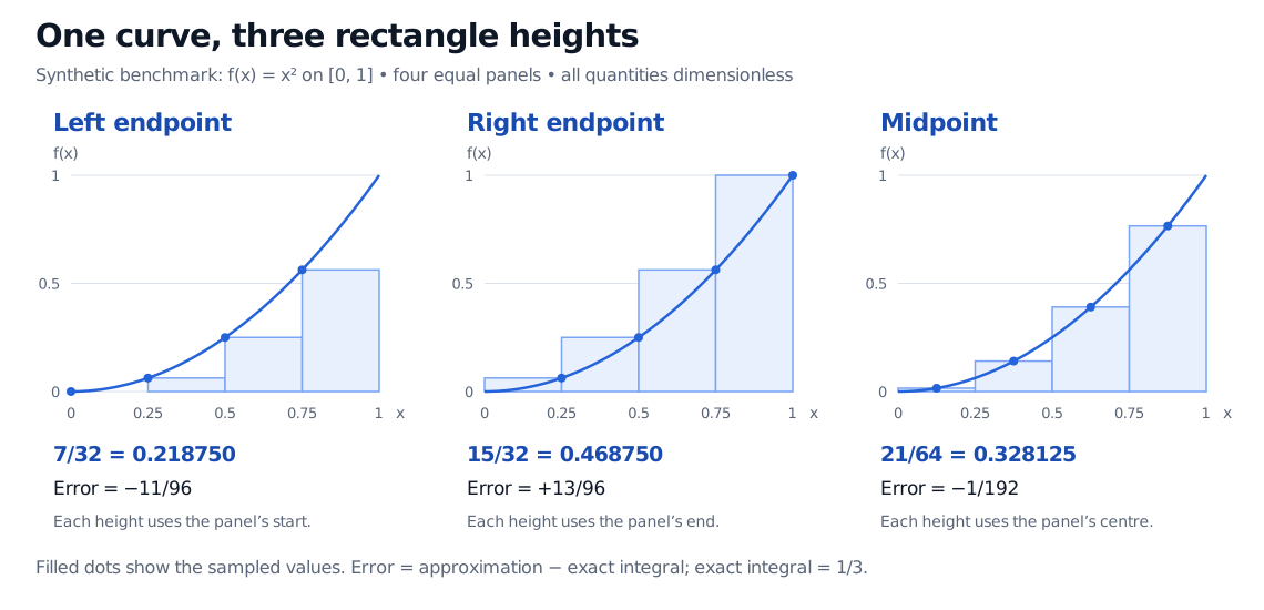
With four panels, $h=1/4$ . The left rule samples $0,1/4,1/2,3/4$ ; the right rule shifts those samples to $1/4,1/2,3/4,1$ . The midpoint rule uses $1/8,3/8,5/8,7/8$ .

Height choice	Approximation	Signed error $Q-I$
Left endpoint	$7/32=0.218750$	$-11/96$
Right endpoint	$15/32=0.468750$	$+13/96$
Midpoint	$21/64=0.328125$	$-1/192$

Three sets of four rectangles for dimensionless x squared on zero to one: left endpoint 7/32, right endpoint 15/32 and midpoint 21/64, compared with the exact integral 1/3.

Original synthetic benchmark. Filled dots identify the sampled heights. Left and right sums bracket this increasing curve; midpoint underestimates this convex curve. Signed errors are approximation minus exact integral.

Here $L_4\le I\le R_4$ because $x^2$ is increasing on this interval. More generally, this bracket holds for an increasing integrand on an ascending partition; a decreasing integrand reverses the inequalities. Positivity is unnecessary: an increasing negative rate is bracketed in the same signed sense. Without monotonicity, endpoint sums need not bracket the integral.

The midpoint underestimate has a different explanation:

x^2

is a convex function. Monotonicity controls the endpoint comparison; curvature controls the midpoint comparison. Do not transfer the left-rule conclusion to the midpoint rule.

Averaging endpoints changes the rule

On the same equal grid, cancellation of the shared interior samples gives

R_n-L_n=h\bigl[f(b)-f(a)\bigr].

Averaging

L_n

and

R_n

produces the trapezoidal rule, not the midpoint rule. In this example that average is

11/32

, whereas

M_4=21/64

. The former averages two endpoint heights; the latter evaluates the function at a new location. Those operations agree for affine functions but generally differ for curved ones.

This distinction matters with recorded data. Endpoint observations do not reveal an unobserved midpoint value. Filling it in requires an interpolation assumption or another observation.

How quickly does the error shrink?

Suppose $f$ is continuously differentiable and $|f'(x)|\le K_1$ on $[a,b]$ . Comparing each endpoint rectangle with its panel's integral gives

|L_n-I|,\ |R_n-I|\le\frac{K_1(b-a)h}{2}.

These are first-order error bounds,

O(h)

. The midpoint bound requires stronger smoothness: if

f

has a continuous second derivative with

|f''(x)|\le K_2

, then

|M_n-I|\le\frac{K_2(b-a)h^2}{24}.

Thus midpoint has second-order error, $O(h^2)$ . Halving the panel width typically halves the leading endpoint error and quarters the leading midpoint error, provided the respective leading terms are nonzero and rounding is negligible. Exactness or cancellation can change an observed ratio. All three rules integrate constants exactly; midpoint also integrates affine functions exactly.

For a cash-flow or payoff integral, retain signed contributions and check whether a jump or kink invalidates the smoothness assumption. More panels reduce discretisation error; they do not supply missing market data or validate the financial model. Composite quadrature develops the broader idea of adding local rules across a partition.

For a derivation from sampled rates to limits, read Areas and Distances: The Riemann Sum. The preview is public; the full lesson requires membership.

Sources

James Stewart, Single Variable Calculus: Early Transcendentals, 6th edition, Thomson Brooks/Cole, 2008, §§5.1–5.2 and §7.7: endpoint sums, midpoint rectangles and error bounds.
Daniel J. Kleitman, Calculus for Beginners and Artists, §14.2, “Rules for Integrating”: endpoint, midpoint and trapezoid constructions.
Joel Feldman, Andrew Rechnitzer and Elyse Yeager, CLP-2 Integral Calculus, §1.11, “Numerical Integration”: midpoint construction and Theorem 1.11.13 on derivative-based error bounds.

Which height are you using?

Three heights for the same curve

Averaging endpoints changes the rule

How quickly does the error shrink?

Sources

Related terms

Composite quadrature

Convex function

Definite integral

Midpoint rule

Trapezoidal rule