Midpoint rule: Definition & Examples

The midpoint rule approximates a definite integral by multiplying an interval's width by the function's value at its centre. The composite version repeats that calculation on smaller intervals and adds the contributions. Each rectangle uses one sampled height.

For a quant, the same construction can approximate an expected payoff against a density or accumulate a changing cash-flow rate. The important choice is where to evaluate the whole integrand. For an expectation, that includes both the payoff and its probability density.

Middle of the interval, not average of the heights

On one interval $[a,b]$ , the approximation is

\int_a^b f(x)\,dx\approx (b-a)f\left(\frac{a+b}{2}\right).

The average happens inside

f

: evaluate the function at the average of the two endpoints. Averaging the endpoint function values instead gives the trapezoidal rule. For

f(x)=x^2

[0,1]

, these heights are

f(1/2)=1/4

and

[f(0)+f(1)]/2=1/2

. They are different calculations. MIT's description of numerical integration rules makes this sampling distinction explicit.

For $n$ equal panels, let $h=(b-a)/n$ and $m_i=a+(i-1/2)h$ . Then

M_n=h\sum_{i=1}^{n}f(m_i).

This is a particular Riemann integral approximation, using the middle of every panel. You need access to those midpoint values: a table containing only the panel endpoints does not provide them without an extra interpolation assumption. An irregular partition is also possible, but each panel then needs its own width and midpoint.

Watching a second moment come into focus

Take the dimensionless benchmark

I=\int_0^1 x^2\,dx=\frac13.

It is also $\mathbb{E}[X^2]$ for a synthetic uniform risk factor $X$ on $[0,1]$ , since its density there is one. This gives a simple exact target for checking an integration routine, rather than a model fitted to financial data.

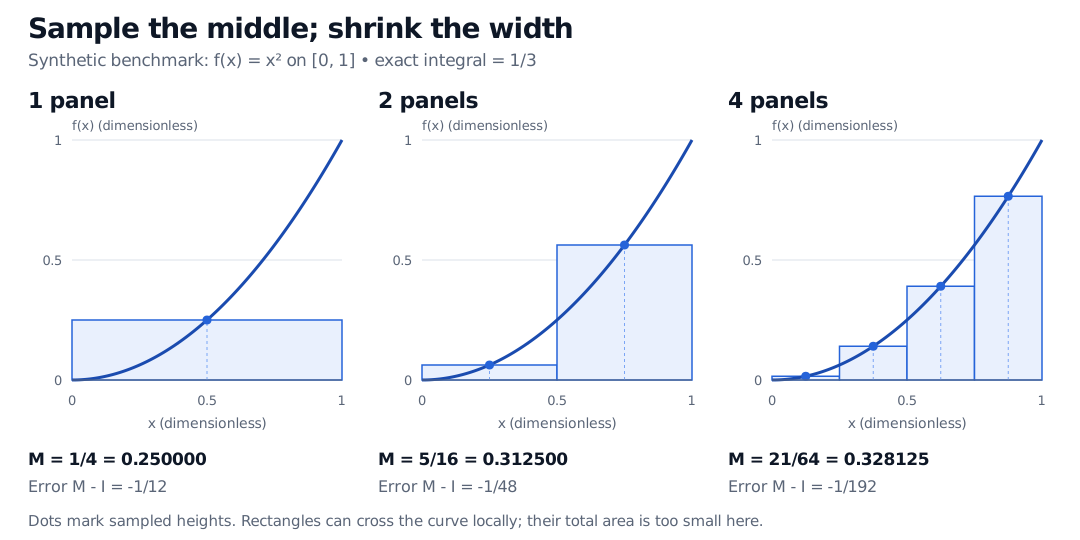
One panel samples $x=1/2$ and gives $M_1=1/4$ . Two panels sample $1/4$ and $3/4$ , giving $M_2=5/16$ . With four panels,

M_4=\frac14\left[\left(\frac18\right)^2+\left(\frac38\right)^2+\left(\frac58\right)^2+\left(\frac78\right)^2\right]=\frac{21}{64}=0.328125.

Midpoint rectangles for dimensionless x squared on zero to one: one panel gives 1/4 with error -1/12, two give 5/16 with error -1/48, and four give 21/64 with error -1/192.

Original synthetic benchmark. Filled dots mark the sampled values. Each doubling of the panel count divides the error magnitude by four; signed errors are approximation minus exact integral.

A rectangle crosses the curve within its panel, so it is not everywhere below it. Its total area is too small here. More generally, midpoint integration underestimates the integral of a convex function on an increasing integration interval, and overestimates for a concave function. Monotonicity alone does not determine this error's sign.

Why curvature matters

At a midpoint $m$ , the linear part of a function is symmetric: its excess on one side cancels its deficit on the other. This makes midpoint integration exact for every affine function, even one with a steep slope.

For our quadratic, write $x=m+s$ on a panel of width $h$ . Direct integration gives

\int_{-h/2}^{h/2}(m+s)^2\,ds=m^2h+\frac{h^3}{12}.

The rectangle retains $m^2h$ and misses $h^3/12$ . On $[0,1]$ , summing over $n$ panels gives the exact law

M_n=\frac13-\frac{1}{12n^2}.

The local error scales as $h^3$ ; the total error on a fixed interval scales as $h^2$ , because the number of panels grows as $1/h$ .

For a general

f

with a continuous second derivative on

[a,b]

, where

a<b

and

\lvert f''(x)\rvert\le K

, the midpoint error bound is

\left|M_n-\int_a^b f(x)\,dx\right|\le\frac{K(b-a)^3}{24n^2}.

Here

K=2

, and the bound equals the actual error magnitude. Usually a bound is more conservative. Second-order convergence describes the smooth refinement regime; it does not promise an exact factor of four for every integrand and panel count, or guarantee midpoint beats every competing rule. Kinks, discontinuities and rounding need separate attention. Composite quadrature compares how several rules behave under refinement.

Keep the units and signs: a rate in USD/year times a panel width in years contributes USD. Negative rates contribute negative amounts. Ordinary midpoint quadrature also assumes an ordinary integral; choosing midpoint samples in a stochastic integral involves different definitions.

For more rectangle geometry and an affine log-return-rate example, read Areas and Distances: The Riemann Sum. Its preview is public; the full lesson requires membership.

Sources

James Stewart, Single Variable Calculus: Early Transcendentals, 6th edition, Thomson Brooks/Cole, 2008, §7.7, “Approximate Integration”: midpoint construction and second-derivative error bound.
MIT, Calculus for Beginners and Artists, §14.2, “Rules” for Integrating: midpoint sampling versus averaging endpoint values.
University of British Columbia, CLP-2 Integral Calculus, §1.11, “Numerical Integration”, especially Theorem 1.11.13 and §1.11.5: midpoint error bound and its local derivation.

Middle of the interval, not average of the heights

Watching a second moment come into focus

Why curvature matters

Sources

Related terms

Composite quadrature

Convergence of a numerical method

Convex function

Definite integral

Trapezoidal rule