Trapezoidal rule: Definition & Examples

The trapezoidal rule approximates a definite integral by joining neighbouring function values with straight lines and integrating those lines. With positive heights, each piece is a trapezoid. The same formula works with negative heights because integration records signed accumulation.

For a quant, it is a transparent baseline for integrating a discounted cash-flow rate or a payoff multiplied by a probability density. It is also useful when only a grid of sampled values is available: the calculation makes an explicit assumption about the behaviour between the samples.

Why the endpoint weights are halved

On one interval $[u,v]$ , integrating the line between $f(u)$ and $f(v)$ gives

\int_u^v f(x)\,dx\approx\frac{v-u}{2}\bigl[f(u)+f(v)\bigr].

This is the interval width multiplied by the average of its two endpoint heights. For

n

equal panels on

[a,b]

, write

h=(b-a)/n

and

x_i=a+ih

. Adding the local contributions gives the composite trapezoidal rule:

T_n=h\left[\frac{f(a)}{2}+\sum_{i=1}^{n-1}f(x_i)+\frac{f(b)}{2}\right].

An interior value belongs to two neighbouring panels, so its two half-weights add to one. Each outer endpoint appears only once. There are $n+1$ sampled values for $n$ panels. A simple average of all sampled heights would give the wrong endpoint weights.

The rule is exact for every affine function: the function already equals its straight-line interpolant. For a curved function it integrates the interpolant exactly, while approximating the original curve.

Seeing the overestimate

Consider the synthetic, dimensionless benchmark

f(x)=x^2,\qquad I=\int_0^1x^2\,dx=\frac13.

It can also represent the second moment of a uniform risk factor on $[0,1]$ , whose density is one. This is a mathematical test case rather than an estimated return model.

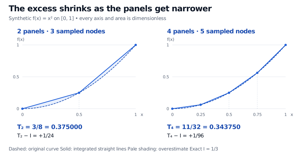
With two panels, the sampled heights are $0$ , $1/4$ and $1$ . The two local contributions are $1/16$ and $5/16$ , giving

T_2=\frac12\left[\frac02+\frac14+\frac12\right]=\frac38=0.375000.

The straight segments lie above the convex curve. Their excess area explains the positive signed error

T_2-I=1/24

Two and four trapezoids above the dimensionless curve x squared on zero to one. Two panels give 3/8 with error plus 1/24; four give 11/32 with error plus 1/96. The exact integral is 1/3.

Original synthetic benchmark. Pale shading is the excess above the curve, solid segments join the sampled heights, and the dashed line is the true integrand. Halving the panel width reduces this quadratic's error by a factor of four.

Panels $n$	Approximation $T_n$	Signed error $T_n-I$
2	$3/8=0.375000$	$+1/24$
4	$11/32=0.343750$	$+1/96$
8	$43/128\approx0.335938$	$+1/384$
16	$171/512\approx0.333984$	$+1/1536$

For this particular quadratic, the exact identity is $T_n-I=1/(6n^2)$ . Consequently $(4T_4-T_2)/3=1/3$ : combining the two approximations cancels their quadratic error. This cancellation is not a universal exact-integration formula; for $f(x)=x^4$ on the same interval, the same combination still has error $+1/1920$ .

What refinement promises

For $a<b$ and a continuous second derivative with $|f''(x)|\le K$ throughout the interval,

|T_n-I|\le\frac{K(b-a)^3}{12n^2}.

The error is therefore $O(h^2)$ on a fixed interval. For the benchmark, $K=2$ and the bound equals its actual error. In general the bound need not be tight, and an observed factor of four under refinement requires a regime dominated by a nonzero second-order error term. Affine exactness, cancellation and rounding can change that pattern.

Convexity gives an overestimate for ascending bounds; concavity gives an underestimate. Neither sign is guaranteed when the curve changes curvature. A payoff kink also breaks the smoothness assumption behind the bound: splitting at the known kink can be more useful than refining an undivided interval. See composite quadrature for how the choice of local rule interacts with the partition.

Keep the grid, units and model separate

For unequally spaced nodes, use each actual width:

T=\sum_{i=1}^{n}\frac{x_i-x_{i-1}}2\bigl[f(x_{i-1})+f(x_i)\bigr].

The equal-spacing formula cannot be applied by pretending irregular observations share one common step. Preserve the order of the nodes: reversing an ascending grid reverses the sign of the integral. Repeated times contribute zero width.

If the integrand is in USD/year and the horizontal variable is in years, each contribution is in USD. Integrating an expected payoff requires the product of payoff and density; adding panels cannot fix an incorrect density, a missing discount factor or omitted tail mass outside a truncated integration window. Nor does a smooth line between noisy observations remove their measurement error.

For a finance-focused continuation, Root-Finding and Numerical Integration develops the trapezoid calculation as an expectation and a pricing input. The preview is public; the full lesson requires membership.

Sources

James Stewart, Single Variable Calculus: Early Transcendentals, 6th edition, Thomson Brooks/Cole, 2008, §7.7, “Approximate Integration”: trapezoidal construction and derivative-based error bounds.
Tobin A. Driscoll and Richard J. Braun, Fundamentals of Numerical Computation, §5.6, “Numerical integration”: integration of piecewise linear interpolation and second-order convergence.
SciPy, scipy.integrate.trapezoid documentation: sampled-data integration, explicit abscissae and reverse integration order.

Why the endpoint weights are halved

Seeing the overestimate

What refinement promises

Keep the grid, units and model separate

Sources

Related terms

Composite quadrature

Convex function

Definite integral