Use random candidate fits and residual thresholds to find a consensus, then distinguish robust refitting from all-point least squares and outlier deletion.
RANSAC
RANSAC (Random Sample Consensus) is a randomized model-fitting method that searches for a large set of observations consistent with one model, then refits using that set. In quantitative research, it can help estimate a relationship when some observations may be grossly corrupted. Its selection rule also creates a risk: a genuine market shock can be excluded simply because it disagrees with the fitted relationship.
The method was introduced by Fischler and Bolles in 1981, for problems involving unreliable measurements and feature matches. It is a fitting strategy, rather than a particular regression equation.
Propose, count, refit
For a straight-line regression, one trial starts with two randomly selected observations with distinct explanatory-variable values. These determine a candidate slope and intercept. Two points with the same explanatory value cannot determine this regression line; they are a degenerate sample.
Next, calculate each observation's residual against the candidate. Observations within a chosen tolerance are inliers; together they form its consensus set. Repeat with other small samples, retain the largest consensus found, and refit on its members. A finite trial budget searches for a large consensus; it does not certify the global maximum.
The scikit-learn algorithm description uses consensus size first and estimator score to break ties, then fits the final model on the chosen inliers. This differs from ordinary least squares, which minimises squared residuals across all observations. Least squares can still be the estimator used inside RANSAC, including for the final refit.
Four points and one large discrepancy
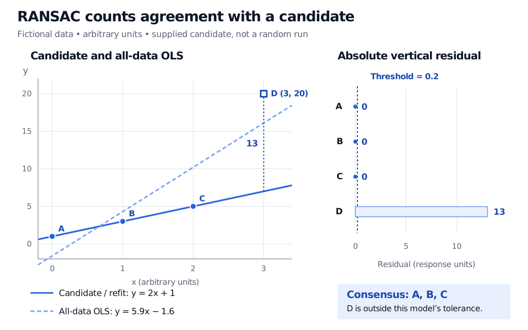
Consider fictional observations in arbitrary units. Take the supplied candidatey^=2x+1 and classify points using an absolute vertical residual threshold of 0.2 response units:
ri=∣yi−(2xi+1)∣,i is an inlier if ri≤0.2.
Observation
x
y
Candidate prediction
Absolute residual
Classification
A
0
1
1
0
Inlier
B
1
3
3
0
Inlier
C
2
5
5
0
Inlier
D
3
20
7
13
Outlier
The consensus contains A, B and C. Refitting least squares to those three points gives the same line, y^=2x+1.
This is a candidate-scoring demonstration, not a reported random run. We can check the search exhaustively here: there are six distinct pairs. Each of the three pairs drawn only from A, B and C gives the supplied line and three inliers. Each pair containing D gives a different line with only its two defining points inside the tolerance. The largest pair-generated consensus therefore has three members.
Fictional points A at (0,1), B at (1,3), C at (2,5) and D at (3,20). The candidate y=2x+1 fits A, B and C exactly; D has vertical residual 13. The all-data OLS line is y=5.9x−1.6. A residual panel marks the 0.2-unit inlier threshold.
Original fictional example. The residual panel uses absolute vertical distances, in response units; its threshold is 0.2. The candidate and its consensus refit coincide.
Fitting OLS to all four points instead gives y^=5.9x−1.6. Its all-point sum of squared errors is 50.7, below the consensus line's 169. That is consistent with the two objectives: OLS wins on all-point squared error, while the supplied candidate wins on the number of points within this tolerance. “Robust” does not mean better under every loss function.
The tolerance defines agreement
The threshold must match the residual definition and its units. Here it is a vertical distance in response units, not the shortest geometric distance to the line. If the response is measured in basis points, an absolute-residual threshold is in basis points too. A squared-residual threshold would instead use squared units.
A tight tolerance can reject legitimate noisy observations; a loose one can accept contamination. Unequal measurement precision may call for scaled residuals rather than one absolute tolerance. The official estimator reference documents the loss, threshold, validity checks and stopping controls; a library default is not a calibration to your data's measurement noise.
More trials buy opportunity, not certainty
An idealised calculation assumes each of s sampled observations is independently an inlier with probability w, trials are independent, and every all-inlier sample yields a valid, useful hypothesis. Under those assumptions,
P(at least one all-inlier sample in N trials)=1−(1−ws)N.
This is an iid sampling calculation, often motivated by sampling with replacement. It excludes degeneracy; repeated observations or poorly arranged points can invalidate the “useful hypothesis” assumption. With distinct observations sampled without replacement from a finite dataset, the single-trial probability differs. In the four-point example, exactly three of six pairs contain only A, B and C, giving 1/2, whereas the iid approximation gives (3/4)2=9/16. Sampling previously untried pairs without replacement also changes dependence across trials.
As the required sample size grows, obtaining a clean sample can become difficult. Competing relationships can produce a large but economically irrelevant consensus. Neither a large iteration limit nor a high nominal stopping probability gives a universal outlier-tolerance or recovery guarantee. For an actual randomized experiment, record the random seed alongside the threshold, loss, sample size and stopping rule.
Finally, an outlier label means disagreement with the chosen model and tolerance. It does not establish a bad tick. Preserve the excluded observations and investigate their provenance and timing. Removing genuine stress events can change the research question from exposure across market conditions to exposure within a selected regime.
For the coefficient and residual calculations behind the refit, see Linear Regression, with a public preview and full teaching available to members.