Range value at risk averages quantiles over a bounded probability band. Calculate discrete cutoff allocations and see why trimming extremes does not guarantee coherent aggregation.
Range value at risk
Range value at risk (RVaR) is the average of a loss distribution's quantiles over a specified probability interval. It summarises losses in a selected band of severity, giving a risk desk a way to average beyond one value at risk threshold while excluding the most extreme tail. That exclusion is a choice about the statistic: the excluded losses remain part of the portfolio's exposure.
Select probability, then average losses
Let L be a one-period loss in a stated currency, with positive values representing losses. Its lower-inverse quantile is
qu(L)=inf{l:P(L≤l)≥u}.
For 0<α<β<1, define
RVaRα,β(L)=β−α1∫αβqu(L)du.
Here α and β are cumulative probability levels, not dollar loss boundaries. The width β−α is the amount of probability selected. RVaR has the same currency and horizon as L; report both levels alongside it. Since quantiles are nondecreasing,
qα(L)≤RVaRα,β(L)≤qβ(L).
The finite interior band is bounded by finite quantiles for a real-valued loss, even when the full upper-tail mean is infinite. This makes RVaR mathematically usable in some heavy-tailed models where expected shortfall is infinite. It does not establish that truncating that tail is economically suitable.
Fifteen percent of scenarios, with the worst five percent left out
Consider this fictional one-day USD loss distribution:
Loss (USD)
Probability
Cumulative probability
0
85%
85%
10
10%
95%
100
5%
100%
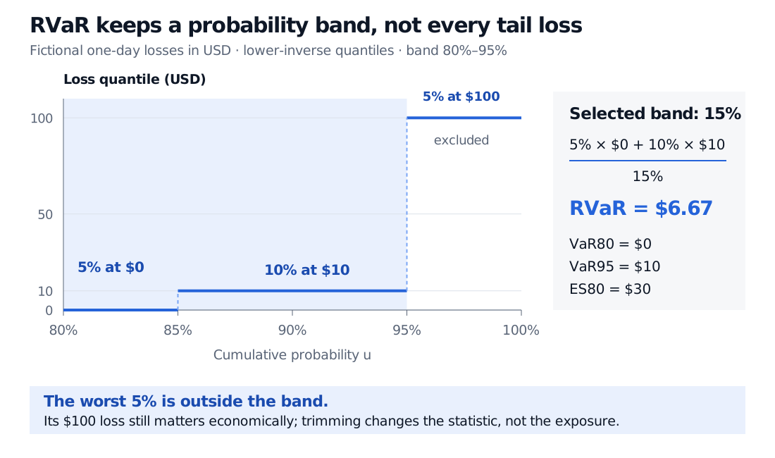
Choose α=0.80 and β=0.95. The quantile is zero through probability 85%, then 10 through 95%, and 100 above 95%. The chosen 15% band therefore contains five percentage points of the zero-loss mass and all ten percentage points of the USD 10 mass:
An equivalent picture uses 100 equally likely ordered scenarios: 85 zeros, ten losses of 10 and five losses of 100. Average scenarios 81 through 95, counting from the smallest loss. The band average is USD 6.67, although no scenario loses that exact amount.
Fictional one-day USD quantile plot from cumulative probability 80% to 100%. The 80%–95% band contains 5% at loss zero and 10% at loss 10, giving RVaR 6.67. The worst 5% at loss 100 is excluded. VaR80 is zero, VaR95 is 10 and ES80 is 30.
Original fictional one-day USD example. The shaded probability band has width 15%; RVaR is the area under the quantile curve within that band divided by its width. The chart omits the first 80% of probability, all at loss zero.
ES80 averages the worst 20%; this RVaR averages the 15% just below the worst 5%. If the USD 100 outcome becomes USD 1,000 with all probabilities unchanged, RVaR stays USD 6.67 while ES80 rises to USD 255. The stable band average and the worsening extreme loss are both true.
Atoms require partial allocation
Averaging observations whose loss amounts lie between two quantile cutoffs can select the wrong probability when there are ties. In this example,
E[L∣0≤L≤10]=0.950.10(10)=1920≈1.05,
while E[L∣0<L≤10]=10. The first conditional expectation includes 95% of the distribution; the second includes 10%. Neither selects the required 15%.
For a finite distribution with ordered distinct losses li and cumulative probabilities ci, where c0=0, a direct calculation is
Each term uses the overlap of that loss's probability interval with the chosen band. This also handles an upper cutoff inside an atom. A single quantile endpoint has zero width and contributes no integral area; an atom occupies a probability interval and can contribute substantial area. Historical and simulated scenario sets need this distinction just as discrete credit-loss models do. A software routine that interpolates sample quantiles estimates a different curve unless that convention is deliberately specified.
For the weighted-average foundations, Expectation, Variance and Covariance works directly from probability weights. The public page is a preview; its full lesson requires a free signed-in account.
Averaging does not guarantee coherence
RVaR respects loss ordering, certain-loss shifts and nonnegative scaling. An interior band is generally not a coherent risk measure because subadditivity can fail.
A separate fictional example makes the problem concrete. Two one-day desk losses each equal USD 10 with probability 4% and zero otherwise. Stipulate that their loss events are mutually exclusive: 92% of scenarios have no loss, 4% only desk A loses, and 4% only desk B loses. Each desk's 80%–95% RVaR is zero because its zero-loss probability is 96%. Their aggregate loss is USD 10 with probability 8%, so its zero-loss probability is 92%:
RVaR0.80,0.95(LA+LB)=0.150.03(10)=2>0+0.
This disproves a universal subadditivity claim at the same probability levels. It does not say aggregation always increases RVaR. Research inequalities that change the band parameters on aggregation do not supply the missing fixed-band guarantee.
When the relevant ES values are finite, splitting the quantile integral gives a useful consistency check:
RVaRα,β=β−α(1−α)ESα−(1−β)ESβ.
For the main example, ES95 is USD 100, so the numerator is 0.20(30)−0.05(100)=1, giving 1/0.15=20/3. The negative ES term is why this is not a positive mixture of coherent measures. Do not use the identity to subtract two infinite ES values; the interior quantile integral can still be finite.
Extending the band to β=1 recovers upper-tail ES when that tail is integrable. Shrinking a band around a point where the quantile function is continuous recovers the point quantile. These relationships explain RVaR's position between a threshold and a tail average without making the measures interchangeable.
Sources
Tobias Fissler and Johanna F. Ziegel, Evaluating Range Value at Risk Forecasts, manuscript version 3, 28 November 2020, §1 and §2.1, especially Definitions 2.1–2.3 and equations (2.2)–(2.3): quantile-band definition, bounds, finite interior bands and atom corrections. The paper uses a gains-positive convention for risk interpretation and lower-tail ES; this article uses positive losses and upper-tail ES.
Paul Embrechts, Haiyan Liu and Ruodu Wang, Quantile-based Risk Sharing, author manuscript dated 24 October 2017, §2 and §3, Theorem 1: risk-measure properties and the distinction between fixed-level subadditivity and aggregation inequalities with changed parameters. Its two parameters describe an excluded tail probability and a band width; this article instead names the two cumulative endpoints. All scenarios, calculations and the figure here are original.