The Rachev ratio compares average upper-tail excess return with average lower-tail loss. Calculate both tails, allocate cutoff probability correctly, and see why the ratio cannot cap losses.
Rachev ratio
The Rachev ratio compares the average excess return in a chosen upper tail with the average loss in a chosen lower tail. It measures the size of unusually good outcomes relative to unusually bad ones, so a strategy can rank differently from one assessed by mean return and volatility. The tail probabilities are part of the measure: a ratio without them is incomplete.
For one stated holding period, define X=R−Rf, where R is the investment's simple return net of the stated costs and Rf is the cash return over the same period. Negative X means underperforming cash; it need not mean a negative total return. The benchmark-adjusted tail-reward/tail-risk construction appears in Ortobelli and coauthors' comparison of performance measures, section 2(l).
Name the probability in each tail
Let qX(u)=inf{x:P(X≤x)≥u} be the quantile function. In this article, α is the upper-tail probability and β the lower-tail probability, both strictly between zero and one. Define
Uα(X)=α1∫1−α1qX(u)du,Dβ(X)=−β1∫0βqX(u)du.
Then
Rα,β(X)=Dβ(X)Uα(X),Dβ(X)>0.
Uα averages the best 100α% of excess returns. Dβ changes the sign of the average of the worst 100β%; it is a positive loss magnitude when that lower-tail average is negative. It does not take an absolute value of every observation or replace returns by their positive parts.
To translate to the common loss-based expected shortfall notation, let ESc(L) average the worst 1−c fraction of losses L, with c a confidence level. Then
Uα(X)=ES1−α(X),Dβ(X)=ES1−β(−X).
In the first expression, X is deliberately fed into the upper-tail loss operator to extract high returns. Thus tail probabilities α=β=0.2 correspond to ES confidence levels of 0.8 for both operators. Do not substitute 0.8 into a formula expecting a tail probability.
Both tail means must be finite. The condition E[∣X∣]<∞ is sufficient. If Dβ=0, division is undefined; if Dβ<0, the lower-tail average is positive and the intended reward-to-loss comparison no longer applies. Report that condition instead of turning the denominator positive. A nonpositive Uα supplies no positive upper-tail reward; divergent tail means do not define a finite performance ratio.
Ten outcomes, two in each tail
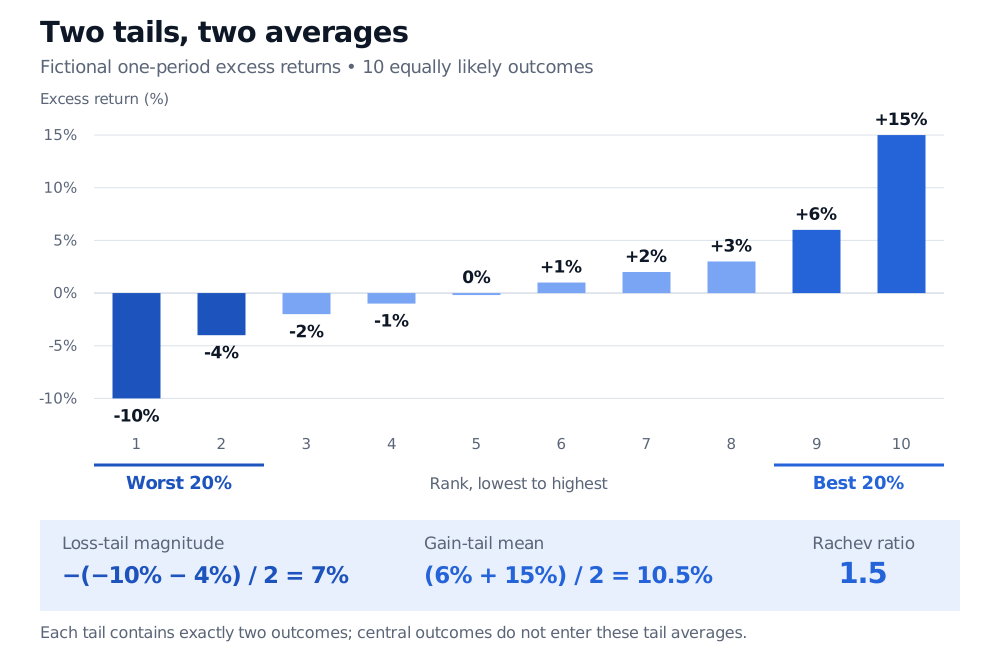
Consider these fictional, equally likely one-period excess returns, with no further cost deduction:
−10%,−4%,−2%,−1%,0%,1%,2%,3%,6%,15%.
Choose α=β=0.2. Each outcome has probability 0.1, so each tail contains exactly two outcomes:
U0.2=26%+15%=10.5%,D0.2=−2−10%−4%=7%.
The ratio is 10.5/7=1.5, a dimensionless number. The average gain in the specified upper tail is 1.5 times the loss magnitude in the specified lower tail. This is neither a win probability nor a promise that gains will cover future losses.
Ten fictional equiprobable excess returns ranked from minus 10% to plus 15%. The worst two average minus 7%; the best two average 10.5%; the Rachev ratio with 20% tail fractions is 1.5.
Original fictional one-period distribution. Each outcome has 10% probability; exactly two outcomes enter each 20% tail. Returns are already measured above cash.
A cutoff is not the whole tail
For this discrete distribution, qX(0.8)=3%. Averaging all observations satisfying X≥3% includes 3%,6%,15%: 30% of the probability, averaging 8%. That is not the best 20% average of 10.5%.
The quantile integrals select exactly the stated probability. If a cutoff crosses an atom, include only the required part of its probability mass. For example, the best 15% here contains the entire 10% mass at 15% and only 5% of the 10% mass at 6%:
U0.15=0.150.10(0.15)+0.05(0.06)=0.12=12%.
This is a weighted average with a fractional boundary allocation, not rounding the requested tail to a whole number of observations. Acerbi and Tasche, Definition 2.6 and Proposition 3.2, establish the tail-mean correction and its quantile-integral representation.
A favourable ratio can still hide an unacceptable loss
Multiply every excess return in the example by two. The upper-tail mean becomes 21%, the lower-tail loss mean becomes 14%, and the ratio remains 1.5. Yet the worst outcome has worsened from −10% to −20%. Positive scaling cancels from the ratio; the ratio alone cannot impose an absolute loss limit. Actual leveraged returns also depend on funding, costs and constraints, which need not scale proportionally.
The Sharpe ratio uses mean excess return divided by its standard deviation. The Omega ratio compares expected positive and negative deviations around a specified return threshold. Neither is this comparison of two selected tail averages; their values and rankings need not agree.
In a backtest, small tails leave few observations to estimate each mean. The ratio can swing because of one gain, one loss, or a denominator near zero. Compare strategies using the same holding period, cash benchmark, cost basis, window, probability weights and tail conventions. Choosing tail probabilities after seeing which values flatter a strategy adds another route to backtest overfitting. Fix the evaluation rule before testing it on held-out data, and inspect the two tail means separately alongside losses and drawdowns.
For the classical measures used in that comparison, Risk-Adjusted Performance Measures develops Sharpe and information-ratio denominators. Its preview is public; the full lesson requires membership.