Quadratic formula: Definition & Examples

The quadratic formula gives the roots of a quadratic equation directly from its coefficients:

ax^2+bx+c=0,\quad a\ne0 \qquad\Longrightarrow\qquad x=\frac{-b\pm\sqrt{b^2-4ac}}{2a}.

Here $a,b,c$ are fixed real numbers. The symbol $\pm$ means evaluate the expression twice, once with addition and once with subtraction; when the square-root term is zero, the answers coincide. The entire numerator is divided by $2a$ .

In quantitative finance, a risk limit can lead to a quadratic equation even when the underlying position depends linearly on hedge size: variance squares the exposure. Two formula roots can then represent very different hedges with the same measured risk.

Why this formula works

The formula packages one operation: complete the square, then undo the square while keeping both signs. Starting from

ax^2+bx+c=0

, multiply by

4a

and move the constant term:

4a^2x^2+4abx=-4ac.

Add $b^2$ to both sides:

\underbrace{4a^2x^2+4abx+b^2}_{(2ax+b)^2}=b^2-4ac.

Write

\Delta=b^2-4ac

, the discriminant. When

\Delta\ge0

2ax+b=\pm\sqrt{\Delta}, \qquad x=\frac{-b\pm\sqrt{\Delta}}{2a}.

This derivation works for either sign of $a$ because $a\ne0$ . If $a<0$ , the “plus” expression need not be the larger root. If $a=0$ , division by $2a$ is invalid; solve the resulting linear or constant equation instead.

The square identity also explains the root count:

\Delta>0

gives two real roots,

\Delta=0

gives a repeated root, and

\Delta<0

gives no real roots. Allowing complex numbers extends the formula to a negative discriminant, but a complex hedge size does not satisfy a real trading constraint.

Two hedge sizes, the same variance

Consider an original synthetic model for P&L over one fixed period. Let $Z$ be a market-factor shock and $E$ a residual shock. Both are dimensionless, have mean zero and variance one, and have zero covariance. No distributional shape is assumed.

Before hedging, the position has three units of factor exposure. Each hedge unit removes one. With dimensionless hedge size $x\ge0$ , suppose

\Delta V_x=1{,}000\big[(3-x)Z+E\big]\,\text{USD}.

This assumes a linear hedge with fixed exposure per unit, no additional hedge noise and no transaction costs. It illustrates algebra, rather than a calibrated trading strategy.

Using the variance rule for a sum, the covariance term vanishes:

\text{Var}(\Delta V_x) =1{,}000{,}000\big[(3-x)^2+1\big]\,\text{USD}^2.

Suppose the target is variance of $5{,}000{,}000\,\text{USD}^2$ , equivalent to P&L standard deviation of approximately USD 2,236.07. Dividing by the fixed scale gives

(3-x)^2+1=5 \quad\Longleftrightarrow\quad x^2-6x+5=0.

Identify $a=1$ , $b=-6$ , $c=5$ . Keep the sign of $b$ inside parentheses when squaring:

\Delta=(-6)^2-4(1)(5)=36-20=16, \qquad x=\frac{6\pm4}{2}.

The two answers are $x=1$ and $x=5$ . An independent check avoids the formula entirely:

(x-3)^2=4

gives

x-3=\pm2

. Substitution into the original variance expression gives

(3-1)^2+1=5

and

(3-5)^2+1=5

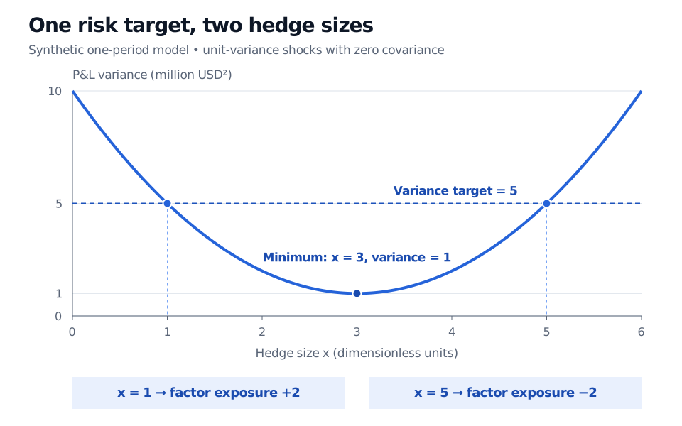
Synthetic one-period P&L variance is 5 million USD squared at hedge sizes x = 1 and x = 5. Their remaining market-factor exposures are +2 and minus 2. Minimum variance is 1 million USD squared at x = 3.

Original synthetic model. Equal variance sits on either side of the minimum-risk hedge. The horizontal axis measures dimensionless hedge units; variance has squared currency units.

x=1

, two positive factor units remain. At

x=5

, the position is overhedged: the factor exposure is

-2

. The equal variances do not establish equal P&L distributions or equal tail risk under the stated assumptions. A positive factor shock moves the two factor components in opposite directions.

Neither answer minimizes variance. The completed-square form shows the minimum at $x=3$ , where factor exposure vanishes and residual variance remains $1{,}000{,}000\,\text{USD}^2$ —standard deviation USD 1,000.

If the target is a cap rather than an equality, all

1\le x\le5

satisfy it, subject to position constraints. If overhedging is prohibited by

x\le3

, only

x=1

meets the target exactly, while

1\le x\le3

stays within the cap. The formula finds equality boundaries; the risk mandate determines how to use them.

From algebra to a calculation you can trust

First put the equation in zero-equals-polynomial form, then identify coefficients, evaluate the discriminant, calculate both branches and substitute into the original model. Check domain restrictions after solving. Useful cross-checks are

x_1+x_2=-\frac{b}{a}, \qquad x_1x_2=\frac{c}{a}.

Here the sum is $6$ and the product is $5$ .

The formula is an exact algebraic identity; a direct computer evaluation can still lose precision when

-b

and

\sqrt{\Delta}

nearly cancel in one branch. See numerical stability for that separate computational issue.

For equation operations and domains, Arithmetic, Algebra, Equations and Functions provides a membership lesson with a public preview. To develop the risk calculation, Expectation, Variance and Covariance is available in full with a free signed-in account; its public page is a preview.

Sources

OpenStax, Algebra and Trigonometry 2e, §2.5, “Quadratic Equations” — completing the square and deriving the formula.
Australian Mathematical Sciences Institute, “The quadratic formula and the discriminant” — real roots and the discriminant.
James Stewart, Single Variable Calculus: Early Transcendentals, 6th edition (2008), Appendix H, pp. A56–A57 — extension of the formula to complex roots.
Dimitri P. Bertsekas and John N. Tsitsiklis, Introduction to Probability, 2nd edition (2008), §4.2, p. 222 — covariance and the variance of a sum.

Why this formula works

Two hedge sizes, the same variance

From algebra to a calculation you can trust

Sources

Related terms

Complex number

Numerical stability

Quadratic equation

Variance