Solve a synthetic trading-profit break-even equation, distinguish its two roots from the profit maximum, and check real roots and feasible quantities.
Quadratic equation
A quadratic equation is an equation that can be written as
ax2+bx+c=0,a=0,
where the coefficients a,b,c are fixed real numbers. Its highest power of the unknown is two. Solving it means finding the values of x that make the equality true, called its roots. A quadratic polynomial is the expression ax2+bx+c; the equation asks when that expression equals zero.
In a financial model, those roots can mark decision boundaries. If expected revenue rises with trade size but execution cost rises with its square, profit can first turn positive and then turn negative again. Finding just one break-even size would miss half the story.
A trade can become too large to break even
Consider an original, synthetic model for one trading opportunity. Let q be quantity divided by one reference lot, so q is dimensionless and q≥0. Suppose expected gross trading profit is 10q USD, execution cost is q2 USD, and a fixed research/setup cost of USD 16 has already been charged to the opportunity. Profit including that setup cost is
Π(q)=(−q2+10q−16)USD.
The fixed charge therefore remains at q=0: this is an accounting convention for the opportunity, not a claim that an uninitiated trade must incur a fee. The numbers illustrate algebra; they are neither observed execution costs nor a fitted market-impact model.
Break-even means Π(q)=0. Divide by the USD unit and multiply both sides by −1:
q2−10q+16=0.
Look for two numbers with sum −10 and product 16. They are −2 and −8, giving
(q−2)(q−8)=0.
A product is zero when at least one factor is zero, so both q=2 and q=8 break even. Direct substitution checks them: −4+20−16=0 and −64+80−16=0.
The factorization also tells us the sign of profit:
Π(q)=−(q−2)(q−8)USD.
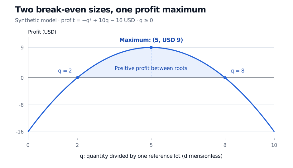
For 2<q<8, one factor is positive and the other negative; the leading minus makes profit positive. For 0≤q<2 or q>8, profit is negative. The two roots bound the profitable region; neither is the profit-maximizing size.
Synthetic profit curve in USD for non-negative dimensionless quantity q. Profit is zero at q = 2 and q = 8, positive between them, and reaches USD 9 at q = 5. At q = 0, profit including the charged setup cost is minus USD 16.
Original synthetic model. Quantity is measured relative to one reference lot. The shaded region has positive profit; the maximum and the break-even points answer different questions.
Completing the square makes that difference explicit:
−q2+10q−16=9−(q−5)2.
A real square cannot be negative, so profit cannot exceed USD 9, achieved at q=5. This finds the maximum without calculus. If a capacity limit permits only 0≤q≤1, neither algebraic break-even root is feasible and all permitted sizes lose money under this model. If only whole reference lots are permitted, evaluate integer quantities; here the break-even quantities happen to be integers.
How many roots should you expect?
For real coefficients, the discriminantΔ=b2−4ac classifies the roots. The quadratic formula calculates them when factoring is inconvenient; it also explains this classification.
Discriminant
Real solutions
Graph of y=ax2+bx+c
Δ>0
Two distinct real roots
Crosses the horizontal axis twice
Δ=0
One repeated real root
Touches the axis at its vertex
Δ<0
No real roots
Never meets the axis
For the normalized break-even equation, a=1, b=−10, c=16, so Δ=100−64=36>0, consistent with two distinct roots. Squaring the negative coefficient matters: b2=(−10)2=100.
A repeated root still counts twice algebraically: (x−3)2=0 has only the single distinct solution x=3. A negative discriminant means no real solution, not no solution in every number system: x2+1=0 has the complex-number roots i and −i. Complex roots cannot represent real trade quantities.
The condition a=0 is essential. If a=0, the equation becomes linear when b=0; if a=b=0, it is either true for every allowed x when c=0, or impossible when c=0. Do not apply a quadratic solver after the squared term disappears.
Preserve solutions, then check the model
Put all terms on one side before identifying coefficients. Factoring a sum does not let you set each original term to zero; the zero-product rule applies to a product equal to zero. Avoid dividing by an expression that might vanish, since that can discard a root.
Finally, substitute every candidate into the original equation and enforce the domain: non-negative quantities, whole lots, capacity limits or any other stated restrictions. Algebra finds model-consistent roots. It does not establish that the assumed revenue and cost curves describe actual trading.
For more on equation operations, units and feasible inputs, see Arithmetic, Algebra, Equations and Functions. Its public page provides a preview; the full lesson requires membership.
James Stewart, Single Variable Calculus: Early Transcendentals, 6th edition (2008), Appendix H, pp. A56–A57 — quadratic roots with negative discriminant and complex conjugates.