How probabilistic programs separate a generative model, conditioning and inference, with an exact regime-signal example and limits of approximate computation.
Probabilistic programming
Probabilistic programming is a way to express a probability model as a program, specify observations, and ask an inference system about the resulting distribution. For a quant estimating an unobserved market regime or uncertain volatility, it separates assumptions about how data arise from the computation used to learn from those data. Random choices and conditioning are central to the formulation described by Gordon, Henzinger, Nori and Rajamani (2014).
One model, three operations
Operation
What it specifies
Generative model
Which quantities are uncertain and how they generate observable data.
Conditioning
Which data have actually been observed; their likelihood changes the relative weights of possible hidden states.
Inference
How to compute the requested conditional probabilities, expectations or other summaries.
A script that merely draws random returns and averages payoffs is a simulation. Randomness alone does not supply the conditioning and inference machinery of a probabilistic programming system. Conversely, inference need not involve random sampling: a small finite model can be solved by enumerating all possibilities.
A positive signal does not set the hidden state
Consider a fictional two-state model, with no fitted market data. Let θ=1 mean stress and θ=0 mean ordinary conditions. Its prior probability of stress is P(θ=1)=0.3. A binary signal Y has these assumed probabilities:
P(Y=+∣θ=1)=0.8,P(Y=+∣θ=0)=0.1.
The generative story draws the regime first, then draws a signal conditional on that regime. Before seeing data, repeatedly running this story describes the joint distribution of regimes and signals.
Now observe Y=+. The likelihood weights the two states differently:
Hidden state
Prior
Likelihood of positive
Unnormalised weight
Stress
0.30
0.80
0.24
Ordinary
0.70
0.10
0.07
The weights sum to the evidence probability, P(Y=+)=0.31. Normalising gives the posterior probability:
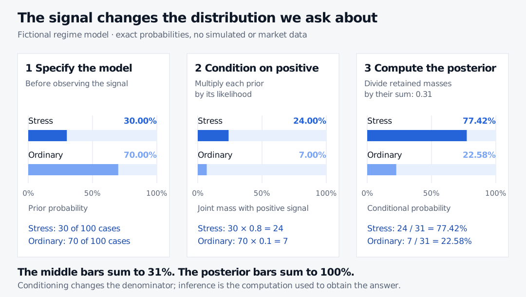
An exact counting interpretation makes the denominator visible: among 100 equally weighted hypothetical cases, 30 are stress cases. Of these, 24 have positive signals; 7 of the 70 ordinary cases also have positive signals. Restricting attention to the 31 positive cases leaves 24 stress cases. The signal raises the stress probability from 30% to about 77.42%, while leaving ordinary conditions possible. The 80% detection probability is a different conditional probability.
Three panels show a fictional model before and after a positive signal. Prior stress and ordinary probabilities are 30% and 70%; positive-signal joint masses are 24% and 7%; dividing by their 31% sum gives posterior probabilities 77.42% and 22.58%.
Original exact model illustration. All bars share a 0–100% scale, but the middle bars are joint masses; only the last panel conditions on the positive signal.
An inference engine still needs checking
Enumeration is exact here. Larger models often require approximation. With Markov chain Monte Carlo, a finite run can explore the posterior poorly, and positively correlated draws contain less information than the raw draw count suggests. Compare multiple chains, inspect traces and convergence diagnostics, and assess effective sample sizes and Monte Carlo standard errors for the quantities being reported. These checks can reveal failures; they cannot prove that a finite run has explored every relevant region. The Stan Reference Manual's posterior-analysis chapter explains both convergence monitoring and sampling precision.
Variational inference instead fits an approximating distribution. A stable optimisation objective does not establish that the approximation captures the posterior's tails or dependence. For example, Stan's ADVI documentation describes a stopping rule based on changes in a noisy objective; that is an optimisation check, not an exactness certificate.
Finally, accurate inference answers the model's question. It does not establish that the prior, signal reliability or regime assumptions describe a changing market. For the underlying updating algebra, Bayesian Reasoning extends this idea to default probabilities and mean returns; its public preview is open, and the full lesson requires membership.