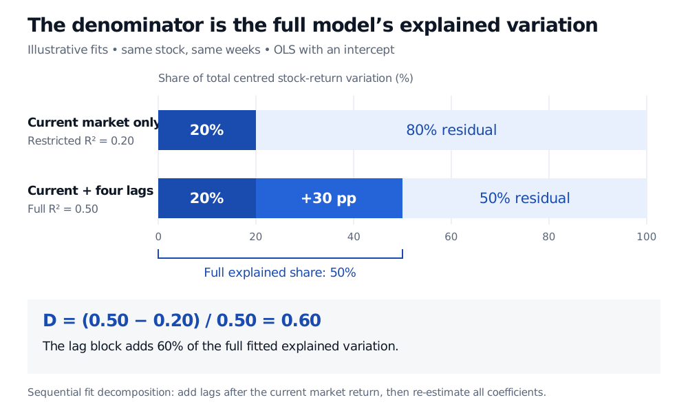
How the Hou–Moskowitz price-delay statistic compares current-market and lagged-market return fits, and why a value of 0.60 is a share of explained variation rather than a response time.
Price delay measure
The price delay measure is a regression statistic that asks how much lagged market returns add to the fit of a stock’s weekly returns, beyond the current week’s market return. A larger value identifies more dependence on past market moves in that fitted specification. For a quant studying information transmission, it is a compact diagnostic of delayed response, rather than a clock measuring how many weeks a price takes to adjust.
Write rj,t for stock j’s return in week t and Rm,t for the market return. The unrestricted model is
rj,t=αj+βjRm,t+k=1∑4δj,kRm,t−k+εj,t.
The restricted model sets all four lag coefficients to zero, retaining an intercept and the contemporaneous market return. Re-estimate the remaining coefficients; do not merely delete fitted lag contributions from the unrestricted model.
In the original 2005 paper, §1.1, the market benchmark is the CRSP value-weighted index. The authors estimate the regression each June using the prior year’s weekly returns. Their weekly observations run Wednesday to Wednesday. The basic statistic is
Both fits must use the same stock-return observations. Build the four lag columns first, handle missing data, and use the resulting common sample in both fits. Otherwise a fit difference can reflect a changed set of weeks rather than the added lag block.
What a value of 0.60 actually says
Suppose, illustratively, the same-sample fits give
Rrestricted2=0.20,Rfull2=0.50.
Then
D1=1−0.500.20=0.60.
The lag block adds 0.30 of total centred return variation, or 30 percentage points of R-squared. That increment is 60% of the full model’s 0.50 explained share. Half of total variation remains unexplained by the full model.
Illustrative same-sample OLS fits: the restricted model explains 20% of total centred stock-return variation; adding four market-return lags raises explained variation to 50%. The incremental 30 percentage points divided by the full 50% explained share gives delay 0.60.
Original illustrative fit decomposition, with total centred variation normalised to 100%. The added fit is conditional on including the current market return first; all coefficients are re-estimated.
The numerator is an incremental fit, not the R-squared of a separate regression on lagged returns alone. Current and lagged market returns may be correlated, so their explanatory contributions are not independent pieces that can be added in any order.
A useful algebraic check uses the common total sum of squares, SST. With residual sums of squares SSEr and SSEu,
D1=SST−SSEuSSEr−SSEu.
The numerator is the reduction in residual squared error from adding lags; the denominator is the full model’s explained sum of squares. Thus 0.60 does not mean that 60% of the stock’s return arrives late, or that adjustment takes 0.60 weeks. The statistic does not identify which lag matters most, and it does not retain the signs of the lag coefficients. Inspect the estimated coefficients when the response pattern matters.
A high estimate needs an explanation
Adding regressors to nested, same-sample OLS cannot worsen the best in-sample fit: the larger model could always choose zero lag coefficients. Ordinary R-squared therefore rises weakly even if the added variables contain no dependable economic information. A positive estimated delay is not, by itself, evidence against market efficiency, a significance test, or a tradable lead-lag strategy.
The mathematical bounds also depend on the convention:
With an intercept, nonconstant stock returns and Rfull2>0, the nested in-sample statistic lies between zero and one. Zero means no improvement from the lag block; one means the current-market-only fit explains nothing while the full fit explains something.
If Rfull2=0, the delay ratio is undefined. A constant response already makes centred R-squared undefined. Very small full-model fit makes a ratio especially sensitive to small fit changes.
Substituting adjusted R-squared, removing the intercept or using out-of-sample scores changes the statistic and its properties. Label such variants explicitly.
The economic interpretation needs more than these identities. Stale prices from thin or nonsynchronous trading can create an apparent lag. Omitted risk exposures or changing coefficients can also make past market returns help a misspecified model. These are competing explanations to investigate, not quantities separated by D1 itself. Hou and Moskowitz discuss frequency-related microstructure concerns in §1 and noisy individual-stock estimates in §1.1.2; their interpretation also assumes relatively stable expected returns over weekly horizons.
For comparisons across stocks or dates, report the market benchmark, weekly endpoints, estimation window, lag count, price and return conventions, sample size, and both underlying R-squared values. Compare results under sensible alternative sampling and model choices, and distinguish statistical evidence from a causal claim about information processing. The contemporaneous market return also makes this a retrospective fit diagnostic; the full regression is not automatically a forecast available before week t begins.
The Linear Regression lesson develops OLS projection geometry, the centred R-squared decomposition and residual checks. Its preview is public; the full lesson requires membership.