The Pástor–Stambaugh liquidity factor measures unexpected changes in aggregate stock-market liquidity, inferred from volume-related return reversals. Its main version is a non-traded liquidity innovation; a separate traded version is a portfolio return. Choosing between them changes what a return regression measures: sensitivity to liquidity shocks or performance relative to a traded benchmark. Pástor and Stambaugh, “Liquidity Risk After 20 Years,” Section 3.1.
Start with a reversal, not a spread
For stock , fit the following within month using daily observations:
Here is the stock's raw return, the value-weighted market return, and dollar trading volume in USD millions. The dependent return and volume sign use returns minus the market, rather than returns minus a risk-free rate. The control remains the raw stock return. Changing it to a market-adjusted return changes the estimator. Original paper, Section II.A, Equation 1.
A negative captures stronger next-day reversal following larger signed volume, holding the raw return fixed. More negative means worse liquidity on this dimension. The sign is an order-flow proxy, rather than observed buyer-initiated minus seller-initiated trades. This is distinct from a quoted bid–ask spread.
Eight observations expose the units
Take eight fictional, nonconsecutive matched-day observations. Each row pairs today's regressors with the following trading day's market-adjusted return. Dollar volume is already signed by today's stock-minus-market return; the table reports raw stock returns in percent and the dependent return in basis points.
| Row | Current raw stock return | Signed volume, USD millions | Next-day stock minus market, bp |
|---|---|---|---|
| 1 | +1% | −2 | 55 |
| 2 | −1% | −1 | 15 |
| 3 | +1% | +1 | −5 |
| 4 | −1% | +2 | −45 |
| 5 | −1% | −2 | 35 |
| 6 | +1% | −1 | 35 |
| 7 | −1% | +1 | −25 |
| 8 | +1% | +2 | −25 |
Convert all returns to decimals before fitting ordinary least squares with an intercept. The exact constructed fit is
For row 1, the fitted decimal return is
The stock can rise 1% while its signed volume is negative: a market rise of 1.5% would leave the stock's market-adjusted return at −0.5%. Signing by the raw return would incorrectly flip that row's volume.
Holding the raw return fixed, an extra positive USD 1 million of signed volume lowers the fitted next-day relative return by 20 bp. At positive USD 2 million, the volume term alone is −40 bp. Neither number is an execution bill or a factor portfolio payoff. Measuring volume in dollars instead of millions would change the coefficient to per dollar, leaving fitted returns unchanged.
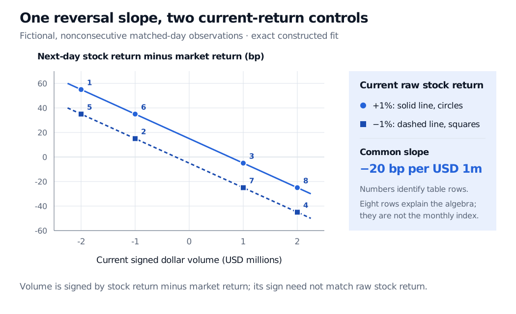
Original fictional regression. Return differences are in basis points; signed dollar volume is in USD millions. The two lines hold the raw-return control at +1% and −1%. Row numbers match the table; the common slope is −20 bp per USD million.
The zero residuals are deliberate arithmetic, with no evidence of predictive skill. Eight rows would fail the original paper's requirement of more than 15 observations for a stock-month. The authors also warn that individual-stock estimates are too noisy for standalone firm-level liquidity measurement; their purpose is aggregation. Original construction; 2019 discussion, Section 3.2.
Four objects that must stay separate
| Object | Construction and meaning |
|---|---|
| Individual | A daily-regression slope for one stock-month; not its liquidity-risk beta. |
| Aggregate liquidity level | Equal-weight average of stock slopes, scaled by ; is the included stocks' total capitalisation at the previous month-end, with August 1962 as the base month. |
| Non-traded innovation | Form same-stock monthly slope differences, then scale; regress on lagged change and lagged scaled level. The normalized residual isolates an unexpected movement. |
| Traded factor, | Value-weighted high-minus-low historical-liquidity-beta decile portfolio return; a different series. |
The innovation construction differences before scaling; simply differencing the scaled level introduces movements from the scaling factor. The paper's Equation 8 divides its fitted residual by 100, an arbitrary normalization affecting beta units. Original paper, Equations 5–8.
An asset's liquidity beta is its return slope on the non-traded innovation, conditional on the chosen other factors. A positive beta means negative liquidity surprises contribute negatively to its fitted return. This return exposure to market liquidity risk differs from liquidity commonality, which concerns liquidity measures moving together. The traded factor instead supports a traded-factor alpha benchmark; it is not designed to track the innovation as closely as possible. 2019 paper, Sections 3.1–3.3.
Read the data column and the timestamp
The author's data file, checked on 31 October 2026, is updated through December 2025. It separates the aggregate level, the non-traded innovation and . The traded series starts in January 1968; earlier entries are the missing-value marker −99, not losses of 99%. is a decimal portfolio return; the other columns are liquidity measures, not investment returns. Retain the distributed normalization and document any conversion rather than applying another automatic percentage adjustment.
A monthly observation label identifies the measurement period, not when a researcher could download or estimate it. A backtest needs the actual data vintage, availability lag and an innovation model estimated with information available at its decision date. Full-sample residuals and revised historical series cannot be assumed to have been observable then. The authors discuss historical CRSP revisions in their 2019 paper, Section 2.
For the next step, Factor Construction separates a characteristic, factor loading and portfolio return. Linear Regression develops fitted slopes, residuals and inference. Both offer public previews; full lessons require membership.
Sources
- Luboš Pástor and Robert F. Stambaugh, “Liquidity Risk and Expected Stock Returns,” original author manuscript, Section II.A, Equations 1 and 5–8; historical-beta portfolio construction in Section III and Table 7. Published in Journal of Political Economy 111 (2003), 642–685.
- Pástor and Stambaugh (2019), “Liquidity Risk After 20 Years”, Sections 2 and 3.1–3.3: revisions, factor choice, noisy firm-level slopes and historical-beta sorts.
- Robert Stambaugh's author data library and liquidity series through December 2025: column definitions, traded-factor construction, dates and missing-value entries.