Partial cointegration models a linear combination of nonstationary time series as the sum of a mean-reverting component and a random walk. In pairs research, this lets a temporary relative-price dislocation coexist with permanent shifts. A large fitted spread therefore need not be a gap that will close completely.
The meaning here is the Clegg–Krauss model used in pairs trading. Ordinary cointegration requires a stationary linear combination of integrated series; partial cointegration allows a stochastic trend to remain in that combination. The word “partial” refers to this decomposition, not a probability that two prices will converge. Clegg and Krauss, §2.1
Two kinds of shock in one residual
For two level series and , each integrated of order one, write a fixed-coefficient relation
Here is a fixed intercept and is a fixed loading. The autoregressive component is transient: the effect of a shock decays with powers of . The random-walk component is permanent: its shocks have no built-in reversal. The basic Gaussian specification takes the two innovation sequences to be mutually independent, zero-mean white noise with variances and . Model definition and intercept convention
With positive random-walk innovation variance, the whole residual is nonstationary, even when is stationary. If , is constant and the residual reduces to a stationary component around a fixed level, given stationary initialization of . This is the full-cointegration boundary. It does not require that fixed level to be zero.
Seven units does not mean seven units will unwind
Consider a fictional current state with , and . The residual is spread units. These component states are stipulated as known for illustration; they are not ordinarily observed separately.
With future innovations having conditional mean zero,
| Horizon | Expected transient component | Expected random-walk component | Expected residual |
|---|---|---|---|
| Now | 2 | 5 | 7 |
| One period | 1 | 5 | 6 |
| Two periods | 0.5 | 5 | 5.5 |
| Three periods | 0.25 | 5 | 5.25 |
| Long-horizon limit | 0 | 5 | 5 |
The transient component has a half-life of period. This is not a half-life for the whole residual. Its conditional expected level tends to 5, not zero. Nor does that forecast mean the realised residual settles at 5: future random-walk shocks continue to accumulate.
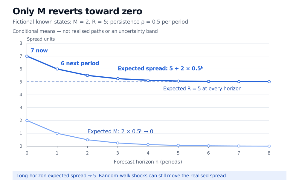
Known-state conditional means with zero-mean future innovations. The chart omits realised shocks and forecast uncertainty; it is not a simulated price path.
A converging conditional mean can coexist with growing uncertainty. Conditional on known current states and fixed parameters, independence gives
The transient contribution is bounded; the random-walk contribution grows with the horizon. This follows by summing the squared innovation weights in the two state recursions. Uncertainty about the current states or fitted parameters requires additional treatment.
The split must be estimated
Observing a residual of 7 does not reveal how much is transient. The authors' approach uses a state-space model, a Kalman filter and maximum likelihood to estimate parameters and hidden components. Filtered states carry estimation uncertainty. A historical smoothed estimate using later observations cannot be treated as a signal available at that earlier date. Authors' estimation and hidden-state documentation
Fitting a decomposition is also different from finding evidence for both components. The authors' documented test framework compares the unrestricted model with pure-random-walk and pure-AR(1) alternatives. An ordinary residual unit-root rejection is not the definition of partial cointegration; a random-walk component is allowed. Boundary hypotheses require appropriate calibration rather than an automatic ordinary likelihood-ratio reference distribution. Authors' testing documentation
For a trade, the relevant candidate dislocation is the estimated transient component. Even if it decays, changes in can overwhelm that movement. Trading results also depend on hedge implementation, transaction costs, borrow availability and stability outside the estimation sample. The model supplies neither zero convergence nor a profit guarantee.
For the contrasting stationary-residual framework, Cointegration and Error Correction develops residual tests and equilibrium adjustment. The preview is public; the full lesson requires membership.
Sources
- Clegg, M. and Krauss, C. (2018), Pairs trading with partial cointegration, Quantitative Finance 18(1), 121–138. FAU publication record; accessible authors' 2016 working-paper version, §§2.1–2.2 and 2.4.
- Clegg, M., Krauss, C. and Rende, J. (2017), partialCI: An R package for the analysis of partially cointegrated time series, §2.1, including the intercept convention.
- Clegg, Krauss and Rende, A partialCI Guide, model, estimation, tests and hidden-state sections. Historical package documentation supports the method; this article does not provide installation instructions.