Understand Type I Pareto tail probabilities, quantiles and moment thresholds through a conditional loss-severity example, and distinguish total losses from Lomax excesses.
Pareto distribution
A Pareto distribution is a continuous probability model whose upper tail decreases as a power of the loss threshold. In the Type I convention used here, a positive minimum xm sets the lower end of the support and a positive shape parameter α controls tail heaviness. A smaller α means more probability far above the minimum.
For a risk analyst, the useful question is often: once a large-loss event has occurred, how large could its loss be? Pareto can model that severity. It does not, by itself, say how often such events occur or supply an annual portfolio-loss forecast.
Specify the minimum before using the formula
For L∼ParetoI(xm,α), with xm>0 and α>0, the survival function is
and zero below the minimum. If L is measured in USD, the density has units of inverse USD. There is no probability atom at xm: the support includes that boundary, but P(L=xm)=0. This is the Type I parameterisation also used by SciPy's Pareto distribution, with zero location and scale xm.
“Power law” refers to the tail's scaling. For any multiplier c≥1 and threshold x≥xm,
P(L>x)P(L>cx)=c−α.
Doubling a threshold therefore multiplies its exceedance probability by the same factor wherever you start above xm. This produces a straight survival curve on logarithmic axes, with slope −α. It is a specific heavy-tailed distribution; heavy tails in general need not follow an exact Pareto law.
A conditional loss-severity example
Suppose a hypothetical operational-risk team models the size of an individual loss, given that it exceeds USD 1,000. Let L denote that conditional severity and stipulate
xm=1,000USD,α=2.5.
These are illustrative assumptions, not estimates from a firm's records. Under this model,
P(L>2,000)=(2,0001,000)2.5=0.1767766953…≈17.68%.
The 17.68% applies among losses already above USD 1,000. To obtain an unconditional exceedance probability for a broader loss variable X, the team also needs P(X>1,000):
P(X>2,000)=P(X>1,000)×0.1767766953….
An annual aggregate-loss model additionally needs event frequencies and assumptions about dependence between events and their sizes. The Loss Distribution Approach lesson develops that frequency–severity distinction and the resulting compound sum. The full lesson requires membership, with a public preview available.
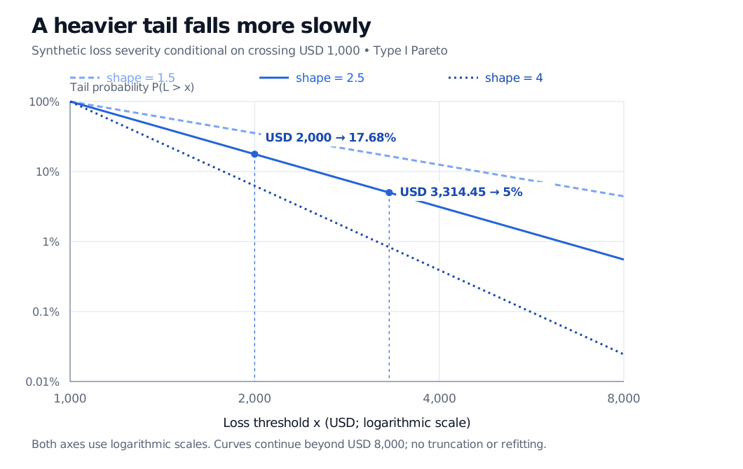
Synthetic conditional Type I Pareto loss severities above USD 1,000, with shapes 1.5, 2.5 and 4. Smaller shape has a heavier tail. For shape 2.5, the probability beyond USD 2,000 is 17.68%, and the probability beyond USD 3,314.45 is 5%.
Original analytical survival curves on logarithmic axes. Minimum USD 1,000 in all three models; only shape varies. The curves continue beyond USD 8,000, and the displayed window does not truncate or renormalise the laws.
Within the conditional severity population, 95% of losses are below that amount and 5% exceed it. A 95th percentile of the full loss population would generally be different.
The losses beyond this threshold can still be much larger. Conditioning a Type I Pareto variable on exceeding q≥xm preserves its shape and replaces its minimum by q. When α>1,
E[L∣L>q]=α−1αq.
At the example's 95th percentile, the average total loss in the upper 5% is therefore USD 5,524.09. The average excess above the threshold is smaller:
E[L−q∣L>q]=α−1q≈2,209.64USD.
Because this law is continuous, its upper-tail conditional mean equals expected shortfall at the same percentile. Here that is expected shortfall of the conditional severity law, rather than of annual aggregate losses. If α≤1, the conditional tail mean is +∞ at every finite threshold; a finite quantile does not make the average beyond it finite.
Which moments actually exist?
For any positive moment order k, integrating the density yields
E[Lk]=⎩⎨⎧α−kαxmk,+∞,α>k,0<α≤k.
The strict inequality matters: the integral still diverges at α=k. In particular,
E[L]=α−1αxm(α>1),Var(L)=(α−1)2(α−2)αxm2(α>2).
Shape
Mean
Variance
0<α≤1
+∞; no finite mean
Undefined under the usual centred definition because there is no finite mean
1<α≤2
Finite
+∞
α>2
Finite
Finite
Our shape of 2.5 gives a mean of USD 1,666.67 and variance of 2,222,222.22 USD-squared, while the third raw moment diverges. Plugging α=1 or 2 into formulas outside their stated domains cannot produce valid moments. A finite observed sample can always have finite numerical averages and variances even when the population moments diverge. See Ross, §5.6.5, and Siegrist's moment derivation.
Type I, Lomax and threshold modelling
The name “Pareto” does not uniquely determine the origin of the variable. For the Type I loss above, the excessY=L−xm begins at zero and has survival function
P(Y>y)=(1+xmy)−α,y≥0.
This is a Lomax distribution, also called Pareto Type II in a common convention. It is a shifted Type I variable, not the same unshifted loss. Its mean is xm/(α−1) when finite, whereas the Type I total-loss mean includes the minimum. SciPy documents the Lomax convention. McNeil, Frey and Embrechts use the zero-origin form in Appendix A.2.8, so check the actual formula before transferring parameters between sources.
The Generalised Pareto and Peaks-Over-Threshold lesson, particularly its definition of the excess variable in §2, develops the broader threshold approach. The full lesson requires membership, with a public preview available. An asymptotic model for excesses above a sufficiently high threshold does not establish an exact Type I law for every loss. Threshold choice, few extreme observations, clustering, reporting cutoffs and actual contractual loss caps all affect whether extrapolating a power law is defensible.
Sources
Sheldon M. Ross, A First Course in Probability, 10th ed., §5.6.5 — Type I construction, density and moment conditions; §6.5, Example 5f — conditioning above a higher threshold.
Alexander J. McNeil, Rüdiger Frey and Paul Embrechts, Quantitative Risk Management: Concepts, Techniques and Tools, revised ed. (2015), §5.2.1 and Appendix A.2.8 — excess distributions and the zero-origin Pareto convention.