A computable substitute for a mathematical value: how approximation error, residuals, tolerances, arithmetic precision and uncertain inputs differ.
Numerical approximation
A numerical approximation is a computable value used in place of a mathematical quantity, with accuracy assessed against a stated target. A quant may approximate an option expectation by a finite sum or solve a bond's yield equation iteratively. The practical question is whether the remaining computational error is small enough for the valuation, hedge or calibration decision.
The target matters. An exact solution of a chosen pricing model can still disagree with the market because the model or its inputs are imperfect. Making the numerical calculation more accurate addresses a different problem.
One candidate, two diagnostics
Take the positive square root x=2 and approximate it by the exact decimal r=1.4142. Its signed approximation error is
r−x=1.4142−2≈−0.000013562373095.
The negative sign means the candidate is too small. Its absolute error is the magnitude of this difference. We can evaluate that error here because the target is independently known to much higher accuracy; in a typical numerical problem, the exact answer is unavailable.
A residual instead asks how well the candidate satisfies the defining equation. For f(z)=z2−2, it is
f(r)=r2−2=1.99996164−2=−0.00003836.
These decimal square and residual values are exact for the stipulated decimal r. They are not the root error. Factoring the difference of squares gives the precise connection:
r−2=r+2r2−2.
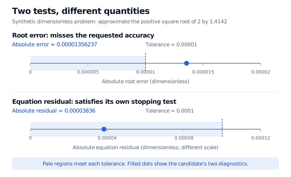
A stopping rule requiring ∣f(r)∣<0.0001 accepts this candidate. A requirement that the absolute root error be below 0.00001 rejects it. Both conclusions are correct: the tests use different quantities and thresholds.
For the approximation 1.4142 to the positive square root of 2, absolute root error about 0.00001356237 exceeds root tolerance 0.00001. Absolute residual 0.00003836 is below residual tolerance 0.0001. The two axes have different scales.
Original synthetic, dimensionless example. Shading marks the values that satisfy each test; filled points are the candidate diagnostics. A residual test and a root-error test answer different questions.
A residual also depends on how the equation is written. Multiplying f by 100 leaves its roots unchanged but changes this residual to −0.003836. Keeping the same residual threshold would change the stopping decision without changing the candidate. For a financial calibration, a price residual may be measured in dollars while the parameter error is measured in yield or volatility points. Converting between them requires information about sensitivity, not just a comparison of decimal places.
What controls the trustworthiness of the answer?
Item
What it describes
What it does not establish by itself
Approximation error
Difference from the mathematical target
Usually unavailable directly when the target is unknown
Residual
Discrepancy in the equation or pricing condition
Small error in the unknown solution
Tolerance
A chosen acceptance threshold for a named quantity
A guarantee unless the method and its assumptions support it
Arithmetic precision
Capacity to represent and operate on numbers
That all displayed digits are accurate
Input uncertainty
Uncertainty in quotes, estimates or measurements
An error removable by running the same calculation longer
An approximation can arise from stopping an iteration, replacing an integral by a finite quadrature sum, or using a finite grid. Floating-point arithmetic introduces another layer: representation and rounding error. More iterations or a finer grid may reduce the mathematical approximation error while eventually exposing roundoff. Accuracy need not improve indefinitely.
A useful solver therefore reports a diagnostic with a defensible interpretation. In exact arithmetic, bisection retains a bracket containing a root; its midpoint is at most half the bracket width from a root in that bracket. That is a bound on root error derived from an interval, rather than an unexplained residual cutoff. In floating-point computation, endpoint evaluation and interval updates also need to be reliable.
For the financial applications, the SelfMadeQuant lesson Root-Finding and Numerical Integration develops scalar solvers and quadrature through yields and expectations. Its preview is public; the full lesson requires membership.
Finally, a more precise output cannot recover information missing from the inputs. Conditioning describes how input changes affect the mathematical answer; numerical stability concerns the algorithm's behaviour. State the target, the error criterion and the input assumptions together before calling an approximation accurate enough.
Sources
Lloyd N. Trefethen and David Bau III, Numerical Linear Algebra, SIAM, 1997, Lecture 14, pp. 102–104, especially “Accuracy”.