A neural ODE learns a continuous vector field and uses numerical integration to transform a hidden state. Separate learned dynamics, solver error and adjoint-gradient accuracy.
Neural ordinary differential equation
A neural ordinary differential equation, or neural ODE, is a model whose hidden-state derivative is parameterised by a neural network. A numerical solver integrates that learned rate of change to produce the output. For a quant modelling observations at uneven times, this offers a continuous latent state between observations—but the numerical solver becomes part of the prediction pipeline.
Here fθ is the learned vector field: given a state and coordinate, it returns the state's instantaneous velocity. The output uses the solution at a chosen terminal coordinate, perhaps followed by a prediction head. Training adjusts θ through a loss on outputs; the solver approximates the trajectory for the current parameters.
A residual network makes a useful connection. A small update of the form
hk+1=hk+Δtfθ(hk,tk)
is a forward Euler step. The neural ODE specifies the continuous field rather than fixing this particular sequence of updates. Its coordinate t can represent network depth; it need not be calendar time. Chen et al. develop both continuous-depth networks and continuous-time latent models.
The same model can give different numerical answers
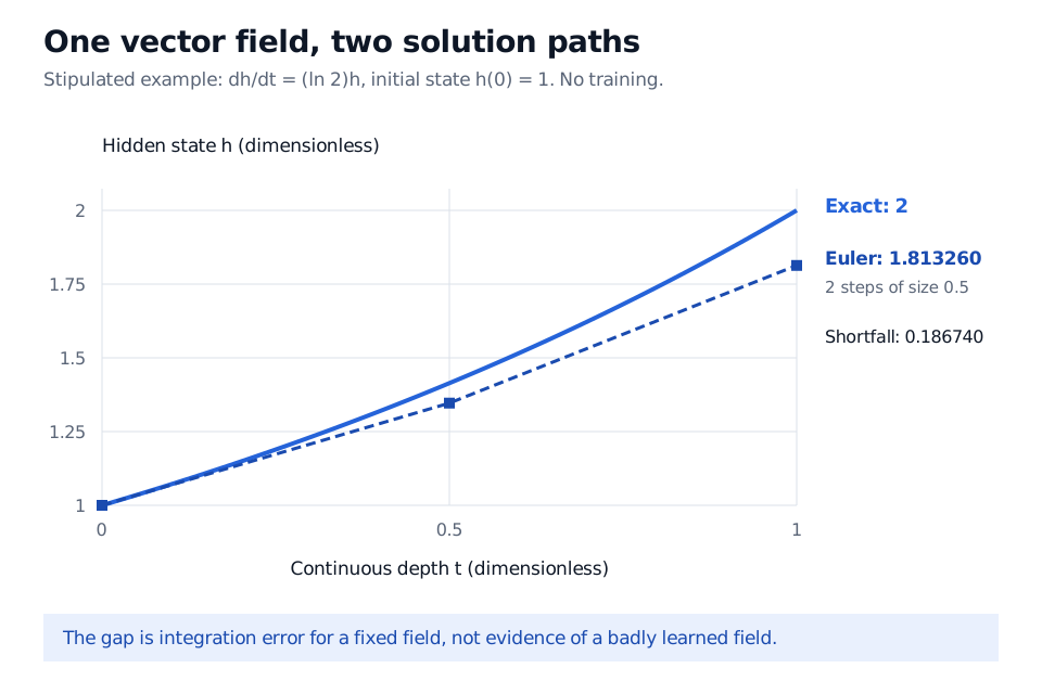
To isolate integration error, stipulate a scalar field with a fixed parameter. Nothing is learned in this example, and both state and depth are dimensionless:
dtdh=θh,h(0)=1,θ=ln2.
Separation of variables gives h(t)=eθt=2t, so h(1)=2. Now approximate the same equation using two forward Euler steps, each of size Δt=0.5:
The terminal shortfall is about 0.186740. That discrepancy is numerical integration error relative to the stipulated equation, not evidence that its parameter was learned incorrectly. Conversely, accurately solving an estimated field does not establish that the field describes financial data well.
Stipulated dimensionless ODE dh/dt equals ln 2 times h, starting at 1. The exact path reaches 2 at depth 1. Two forward Euler steps of size 0.5 reach 1.813260, a shortfall of 0.186740, with the vector field held fixed.
Original stipulated scalar example, with no fitted data. The solid curve is the exact solution; square markers and dashed segments show two forward Euler steps. All states and depth coordinates are dimensionless.
As the authors' torchdiffeq documentation explains, solver method, step size and adaptive tolerances trade computation against numerical accuracy. Tolerances control numerical error estimates, not statistical prediction error. Forward and backward settings both matter during training. Chen et al., §6 discusses this choice and trajectory-reconstruction error.
The continuous adjoint method propagates loss sensitivities through another differential equation solved backwards; the authors' implementation documentation describes this exchange of storage for a backward solve. Avoiding storage of every forward solver step can reduce activation memory. This is a claim about storage relative to integration steps, not zero memory or free computation.
There are two distinct accuracy issues. Reconstructing the forward state by integrating backwards may amplify numerical error; mathematical uniqueness does not guarantee a stable numerical reversal. Also, discretising continuous sensitivity equations need not give the exact gradient of the discretised forward calculation. ANODE, §§III–IV analyses these problems and uses checkpointing with differentiation of the discretised computation. Checkpoints trade storage and recomputation for reliable access to forward states. Gradient checks must therefore target the calculation actually being trained; calling a solver a black box does not make its numerical gradients exact.
A continuous clock does not enforce an information clock
For financial forecasting, an initial-state encoder must use only information available at the forecast origin. An encoder that reads the entire realised sequence can be useful for retrospective reconstruction, but feeding its state into a claimed historical forecast introduces look-ahead bias. Continuous integration does not remove that distinction.
A deterministic neural ODE also has no fresh random shocks once its parameters and initial state are fixed. Random initial states or observation noise can provide uncertainty in a larger model; a stochastic differential equation instead includes a stochastic driving process. Neither irregular timestamps nor continuous depth alone establishes a causal mechanism or a profitable trading signal.