Maximum mean discrepancy: Definition & Examples

Maximum mean discrepancy (MMD) measures how far apart two probability distributions are after mapping observations into a kernel’s feature space and taking the mean of each group. A quant can use it to monitor data drift by comparing a reference sample of model inputs with a recent one. For example, the joint behaviour of bid–ask spreads and quoted depth could change even if each input’s average holds steady.

What the kernel can see

A kernel computes an inner product

k(x,y)=\langle\phi(x),\phi(y)\rangle_{\mathcal H}

between feature representations. When the population mean embeddings

\mu_P=\mathbb E_P[\phi(X)]

and

\mu_Q=\mathbb E_Q[\phi(Y)]

exist, MMD is the distance between them. The name comes from an equivalent view. Among functions in the unit ball of the reproducing kernel Hilbert space

\mathcal H

, it finds the largest gap in average function values.

\begin{aligned} \operatorname{MMD}_k(P,Q) &= \lVert\mu_P-\mu_Q\rVert_{\mathcal H}\\ &= \sup_{\lVert f\rVert_{\mathcal H}\le 1} \bigl|\mathbb E_P[f(X)]-\mathbb E_Q[f(Y)]\bigr|. \end{aligned}

The norm constraint fixes the scale of the functions being compared. The kernel determines which differences those functions can detect. A characteristic kernel gives different population embeddings to different distributions, so population MMD is zero exactly when

P=Q

. The Gaussian radial basis function kernel is characteristic on

\mathbb R^d

at any fixed positive bandwidth. A linear kernel retains only the ordinary mean vector. Gretton et al., §2, Sriperumbudur et al., Theorem 9 and §6.

The SelfMadeQuant lesson The Kernel Trick: Feature Maps and Properties of Kernels shows how to compute these inner products without forming the feature vectors. The full lesson requires membership.

Two samples with the same mean

For

m

observations

x_i

and

n

observations

y_j

, the biased empirical squared MMD expands the squared distance between the two sample embeddings. Compute the average kernel value within each sample, add those two averages and subtract twice the average across samples.

\begin{aligned} \widehat{\operatorname{MMD}}_{b,k}^{\,2} ={}&\frac{1}{m^2}\sum_{i,j=1}^{m} k(x_i,x_j) +\frac{1}{n^2}\sum_{i,j=1}^{n} k(y_i,y_j)\\ &-\frac{2}{mn}\sum_{i=1}^{m}\sum_{j=1}^{n} k(x_i,y_j). \end{aligned}

The within-sample sums include the diagonal, so each observation is compared with itself. The result is nonnegative because it is a squared norm. Under independent sampling, the noise in the sample embeddings contributes an upward bias to the squared distance. With two independent samples of at least two i.i.d. observations each, one unbiased estimator of population squared MMD drops the within-sample diagonals, divides those sums by

m(m-1)

and

n(n-1)

, and retains all cross-sample pairs. Distinct observations with the same value still count as off-diagonal pairs. That estimator can be negative in a finite sample. Gretton et al., §2.2, equations (3) and (5).

Use the linear kernel $k(x,y)=xy$ and take three fictional samples, $A=(0,2)$ , $B=(2,4)$ and $C=(1,1)$ . With all pairs included, each kernel average factorises into a product of sample means. For $A$ and $B$ , the squared score is $1+9-6=4$ , the same as $(1-3)^2$ . For $A$ and $C$ , it is $1+1-2=0$ . Both means are $1$ , although $A$ puts half its mass on each of $0$ and $2$ , while $C$ puts all its mass on $1$ . With the unbiased formula, the within-sample average for $A$ falls from $1$ to $0$ , and the squared MMD estimate for $A$ versus $C$ is $-1$ .

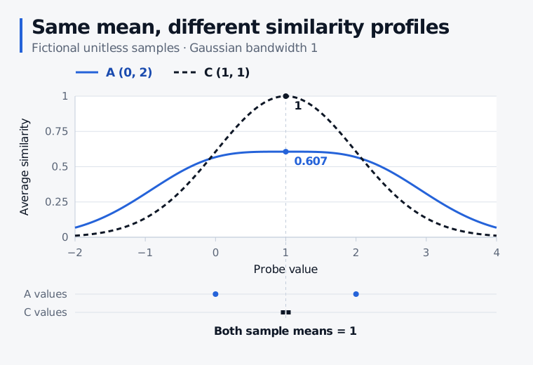
Keep $A$ and $C$ , but use the Gaussian kernel $k(x,y)=\exp(-(x-y)^2/2)$ with bandwidth $1$ . The mean similarity to a probe at $1$ is $e^{-1/2}$ for $A$ and $1$ for $C$ . The mean similarity profiles therefore differ even though the raw means agree. With the Gaussian kernel the same biased squared calculation gives

\widehat{\operatorname{MMD}}_{b,k}^{\,2} = \tfrac32+\tfrac12 e^{-2}-2e^{-1/2} \approx 0.3546.

Fictional unitless samples A (0, 2) and C (1, 1) share a mean of 1. At probe value 1 their Gaussian mean similarities are 0.607 and 1. Their biased squared MMD is 0 with the linear kernel and 0.3546 with the Gaussian kernel at bandwidth 1.

Each curve shows the sample’s average Gaussian similarity to a probe value. The solid curve is higher near the ends of the plotted range. The dashed curve peaks at the common mean.

When the score becomes a test

To turn an observed score into a hypothesis test of

P=Q

, compare it with a null distribution. Even when two samples come from the same population, their empirical embeddings usually differ. With independent i.i.d. samples and a fixed kernel, the observations are exchangeable under the null. A permutation test pools the observations, repeatedly reallocates them to groups of the original sizes and recomputes the same statistic. The fraction of scores at least as large as the observed score, counting the original assignment, gives a permutation p-value. Bandwidth affects which differences the test has power to detect. If group labels are used to tune the kernel, one valid design is to do that on separate training data and run the permutation test on untouched observations. Biggs, Schrab and Gretton, §§1–2.

For a trading model, consecutive feature rows may share underlying observations because their lookback windows overlap. Shuffling individual rows breaks that dependence, so a null calibrated that way can give misleading alerts. Dependence-aware calibration has to match the window design, including any dependence between windows. One published wild-bootstrap MMD result covers independent stationary series with sufficiently fast decay of dependence within each series, using a bounded Lipschitz kernel. Adjacent windows cut from one series can fall outside that setup. Chwialkowski, Sejdinovic and Gretton, §4.1.

A rejection on spread and depth concerns the distribution of those inputs. Evaluating whether the model’s forecasts or execution decisions have deteriorated requires outcome data.

Sources

Gretton et al. (2012), A Kernel Two-Sample Test, §§2–3.
Sriperumbudur et al. (2010), Hilbert Space Embeddings and Metrics on Probability Measures, Theorem 9 and §6.
Biggs, Schrab and Gretton (2023), MMD-FUSE: Learning and Combining Kernels for Two-Sample Testing Without Data Splitting, §§1–2.
Chwialkowski, Sejdinovic and Gretton (2014), A Wild Bootstrap for Degenerate Kernel Tests, §4.1, Proposition 1.

What the kernel can see

Two samples with the same mean

When the score becomes a test

Sources

Related terms

Hypothesis test

Kernel method and kernel trick

P-value

Radial basis function kernel