How the Gaussian RBF kernel turns feature distance into similarity, why gamma depends on scaling, and what kernel validity does—and does not—guarantee.
Radial basis function kernel
A radial basis function kernel measures similarity using only the distance between two inputs. In machine learning, “the RBF kernel” usually means the Gaussian RBF kernel: nearby feature vectors receive a value close to one, while distant vectors receive a value close to zero. For a quant comparing market states, the consequential choice is what counts as nearby. Feature units and scaling can change that answer before a model learns anything.
The Gaussian convention
For vectors x,y∈Rd, the Gaussian kernel is
kγ(x,y)=exp(−γ∥x−y∥2),γ>0.
Here ∥x−y∥ is Euclidean distance in the coordinates supplied to the model. The kernel equals one when the inputs coincide and lies strictly between zero and one otherwise. Larger γ makes similarity decay over shorter distances. The official pairwise-kernel definition uses this convention.
The same Gaussian is often written using a length scale ℓ>0:
k(x,y)=exp(−2ℓ2∥x−y∥2),γ=2ℓ21.
A large length scale therefore means a small gamma. Do not transfer their numerical values unchanged between parameterisations. Rasmussen and Williams, §4.2.1, use the length-scale form.
“Radial” is broader than “Gaussian”: it describes dependence on distance alone. Other valid radial kernels include the exponential kernel exp(−∥x−y∥/ℓ). A function does not become a valid machine-learning kernel merely because it is radial or decreases with distance.
Same pair, different geometry
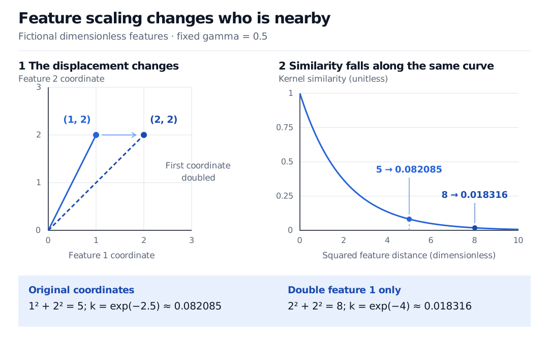
Consider two fictional market-state observations represented by dimensionless transformed features. Their coordinate differences are 1 and 2. With γ=0.5,
∥x−y∥2=12+22=5,k(x,y)=e−2.5≈0.082085.
Now double the first coordinate of every observation, leaving the second unchanged and holding gamma fixed. The differences become 2 and 2:
∥x−y∥2=22+22=8,k(x,y)=e−4≈0.018316.
The underlying observations have not changed. Their representation has made the first feature count four times as much in squared distance. A single adjustment to gamma cannot generally undo a change in only one coordinate for every possible pair.
Fictional dimensionless feature displacement changes from (1, 2) to (2, 2) when feature 1 is doubled. With gamma fixed at 0.5, squared distance rises from 5 to 8 and Gaussian RBF similarity falls from 0.082085 to 0.018316.
Original fictional example. Reweighting one coordinate moves the pair along the same Gaussian kernel curve; it changes similarity even though gamma stays fixed.
This is why a return expressed in percentage points and a spread expressed in basis points should not be thrown into Euclidean distance without a deliberate scaling rule. Gamma has inverse squared-distance units; its numerical meaning belongs to the chosen coordinate system.
Standardising features can remove arbitrary scale differences, but it does not establish that equal standardised distances are equally informative. If using estimated means and scales, fit them on the training portion of each validation split, then apply those fixed transformations to its validation portion. Estimating scales from the full sample leaks held-out information into the geometry. This follows the official preprocessing and leakage guidance.
Similarity is an ingredient, not a forecast
For any finite collection of Euclidean inputs, the Gaussian RBF produces a symmetric positive semidefinite matrix with entries Kij=k(xi,xj). This is the validity property needed to use it as an inner-product kernel. It supports nonlinear learning through the kernel method, without explicitly constructing its feature coordinates. See GPML §4.1 for the finite-matrix criterion; the matrix-characterisations lesson develops the underlying quadratic-form test (public preview; full lesson requires membership).
A similarity of 0.082085 is not an 8.2% probability that two observations share a regime. Nor is this unnormalised Gaussian-shaped function a probability density or a likelihood. Kernel ridge regression must still learn coefficients and choose its penalty. A Gaussian process can use the kernel as a covariance component, but its probabilistic predictions additionally require a mean, an amplitude convention and an observation model. The official GP regression documentation separates the prior covariance from the likelihood and noise specification.
At the extremes, for a fixed finite data set:
As γ→0, every entry approaches one: the kernel loses its ability to distinguish inputs.
As γ→∞, similarity approaches zero between distinct inputs and stays one between identical inputs. The training matrix approaches the identity only if the inputs are all distinct.
These limits explain why gamma controls locality; they do not identify an optimal setting. Select gamma together with the model's regularisation using cross-validation appropriate to the prediction task. For market data, preserve the information available at each forecast date and account for overlapping labels. Keep the final test period out of selection. The official RBF SVM example illustrates how gamma and the penalty interact. Mathematical kernel validity alone guarantees neither predictive accuracy nor a tradable signal.