Kernel ridge regression: Definition & Examples

Kernel ridge regression (KRR) fits a response function by minimizing squared prediction errors plus a penalty on its size in a kernel-defined function space. It extends ridge regression to nonlinear relationships without explicitly building every transformed feature. A quant could use it to model execution cost from order size, spread and volatility; the kernel determines which combinations of those inputs the model treats as similar. Nonlinear flexibility does not itself establish predictive value. scikit-learn, §1.3

A fit expressed through training observations

Given training pairs

(x_i,y_i)

, choose a real symmetric kernel

k

. It must generate a positive semidefinite matrix for every finite collection of inputs, not merely assign plausible similarity scores. Write

K_{ij}=k(x_i,x_j)

. This is the training Gram matrix; it can be rank deficient, for example when feature representations repeat. Rasmussen and Williams, §4.1

Let $\mathcal H_k$ be the kernel's reproducing kernel Hilbert space (RKHS): the function space with a norm compatible with evaluating functions through $k$ . Here the objective is

\widehat f=\arg\min_{f\in\mathcal H_k} \left\{\sum_{i=1}^{n}(y_i-f(x_i))^2+\lambda\lVert f\rVert_{\mathcal H_k}^{2}\right\}, \qquad \lambda>0.

The loss is an unaveraged sum and there is no separate unpenalized intercept. The norm measures function size according to the chosen kernel; it is not generally the squared Euclidean norm of the kernel coefficients. The representer theorem reduces the fit to

\widehat f(x)=\sum_{i=1}^{n}\alpha_i k(x_i,x), \qquad (K+\lambda I_n)\alpha=y.

For this representation,

\lVert f\rVert_{\mathcal H_k}^{2}=\alpha^\top K\alpha

. Replacing that term by

\alpha^\top\alpha

changes the problem. A positive

\lambda

makes

K+\lambda I_n

positive definite even when

K

is singular. The displayed system gives a unique coefficient vector; for singular

K

, other coefficient representations can describe the same fitted function. Rasmussen and Williams, §§6.1–6.2.2

Check the normalization before copying a penalty setting. If the objective instead uses

n^{-1}\sum_i(y_i-f(x_i))^2+\lambda\lVert f\rVert_{\mathcal H_k}^{2}

, its system is

(K+n\lambda I_n)\alpha=y

. Keeping the same fit therefore requires dividing the unaveraged-loss penalty by

n

. Multiplying the entire objective by a constant changes no minimizer; scaling only one term does.

Two observations, one coupled solution

Take fictional, unitless responses and a valid kernel matrix:

K=\begin{pmatrix}1&0.5\\0.5&1\end{pmatrix}, \qquad y=\begin{pmatrix}1\\0\end{pmatrix}, \qquad \lambda=0.5.

Its eigenvalues are $1.5$ and $0.5$ , both positive. One explicit feature construction is $\phi(x_1)=(1,0)^\top$ and $\phi(x_2)=(0.5,\sqrt{0.75})^\top$ , using $k(x,z)=\phi(x)^\top\phi(z)$ . Their inner products reproduce $K$ , so the example can also be checked by ordinary ridge regression in these two features.

The kernel system is

\begin{aligned} 1.5\alpha_1+0.5\alpha_2&=1,\\ 0.5\alpha_1+1.5\alpha_2&=0, \end{aligned} \qquad \alpha=\begin{pmatrix}0.75\\-0.25\end{pmatrix}.

The fitted training values are not the coefficients:

\widehat y=K\alpha =\begin{pmatrix}0.75-0.125\\0.375-0.25\end{pmatrix} =\begin{pmatrix}0.625\\0.125\end{pmatrix}.

The negative second coefficient offsets the positive similarity between observations. These coefficients are not probabilities or portfolio weights. At a new input $x_*$ , prediction requires its similarities to the training inputs: $\widehat f(x_*)=k_*^\top\alpha$ , where $(k_*)_i=k(x_i,x_*)$ . The training matrix alone does not specify every future prediction.

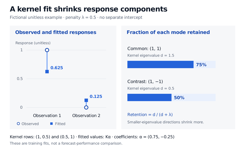
Fictional unitless responses 1 and 0 become fitted values 0.625 and 0.125 at penalty 0.5. Kernel eigenvalues 1.5 and 0.5 retain 75 percent of the common-response component and 50 percent of the contrast component.

Original deterministic example, with no separate intercept. The two observations are categories, not positions on a fitted curve. The right panel shows the fraction retained along each kernel eigenvector.

Why do the responses move this way? For an eigenvector of $K$ with eigenvalue $d$ , the training smoother $K(K+\lambda I_n)^{-1}$ retains the fraction $d/(d+\lambda)$ of that response component. Here the common direction $(1,1)^\top$ retains $75\%$ , while the contrast direction $(1,-1)^\top$ retains $50\%$ . Thus

y=0.5\begin{pmatrix}1\\1\end{pmatrix} +0.5\begin{pmatrix}1\\-1\end{pmatrix} \quad\longrightarrow\quad \widehat y=0.375\begin{pmatrix}1\\1\end{pmatrix} +0.25\begin{pmatrix}1\\-1\end{pmatrix}.

This is joint regularization, rather than the normalized local average used in Nadaraya–Watson kernel regression. KRR need not have nonnegative response weights or weights summing to one. With no separate intercept, even a constant response component can shrink, as the common direction does here.

What a financial prediction still needs

For a distance-based kernel such as a radial basis function kernel, feature units and scale affect similarity. Fit preprocessing on each training fold, apply that fitted transformation to its validation data, and select kernel parameters and the penalty within the training portion of the evaluation design. Leave the final test period untouched by selection. These steps prevent the preprocessing and tuning forms of look-ahead bias. scikit-learn, §§12.1–12.2.1

For financial time series, preserve forecast chronology and ensure training labels are available at the forecast origin; overlapping future-return labels can require purging around validation boundaries. Use cross-validation that reflects the intended deployment. The small training calculation above measures neither future forecast error nor returns after trading costs.

KRR supplies a point prediction, not an uncertainty band. A zero-mean Gaussian process regression model has the same posterior mean when its covariance kernel matches

k

, its independent Gaussian observation-noise variance equals this unaveraged-loss

\lambda

, and the data transformations match. That correspondence does not establish calibrated uncertainty for actual market data. Rasmussen and Williams, §2.2, equations 2.25–2.27

For a dense exact implementation, storing the Gram matrix takes

O(n^2)

memory and a standard factorization takes

O(n^3)

work. Solve the regularized linear system, for example by Cholesky factorization, rather than explicitly forming an inverse. A new prediction generally uses all

n

kernel evaluations; this is not ordinarily a sparse model. Rasmussen and Williams, Algorithm 2.1, scikit-learn, §1.3

For the feature-map intuition behind this construction, see The Kernel Trick: Feature Maps and Properties of Kernels (public preview; full lesson requires membership).

Sources

Rasmussen and Williams, Gaussian Processes for Machine Learning, §§6.1–6.2.3: RKHS norms, representer theorem and squared-error regularization.
Rasmussen and Williams, §4.1: valid kernels and positive semidefinite Gram matrices.
Rasmussen and Williams, §2.2 and Algorithm 2.1: matched Gaussian-process mean and stable linear-system computation.
scikit-learn User Guide, §1.3: kernelized ridge regression and its generally dense prediction representation.
scikit-learn User Guide, §§12.1–12.2.1: consistent preprocessing and training-only fitting of transformations.

A fit expressed through training observations

Two observations, one coupled solution

What a financial prediction still needs

Sources

Related terms

Look-ahead bias

Nadaraya–Watson kernel regression

Positive semidefinite matrix

Radial basis function kernel

Representer theorem