Representer theorem: Definition & Examples

The representer theorem says that, for a broad class of regularised learning problems in a reproducing kernel Hilbert space, every minimising function can be written as a finite sum of kernels centred at the training inputs. For a quant fitting a nonlinear signal or response surface, this turns a potentially infinite-dimensional function search into an optimisation over finitely many scalar coefficients. It does not establish that the fitted signal will predict future returns.

The statement needs an objective

Let $\mathcal H$ be a real reproducing kernel Hilbert space (RKHS) with kernel $k$ . Fix training inputs $x_1,\ldots,x_n$ and their labels. Consider

\min_{f\in\mathcal H} J(f),\qquad J(f)=L\bigl(f(x_1),\ldots,f(x_n)\bigr)+\Omega(\lVert f\rVert_{\mathcal H}),

where the labels are held fixed inside $L$ . Assume a finite-valued global minimiser exists and $\Omega$ is strictly increasing on $[0,\infty)$ . Then every global minimiser has the form

f^*(x)=\sum_{i=1}^{n}\alpha_i k(x_i,x),\qquad \alpha_i\in\mathbb R.

The loss can couple the evaluations and need not be a sum of squared errors. Strict increase concerns the RKHS norm, not an arbitrary penalty on a software parameter vector. The theorem describes existing minimisers; it does not prove existence or make a nonconvex loss easy to optimise. If

\Omega

is merely nondecreasing, projection still yields at least one minimiser of this form, assuming a minimiser exists, but other minimisers may lie outside the span. Schölkopf, Herbrich and Smola, §2, Theorem 1 and following remarks

Why the unseen directions disappear

Set

S=\operatorname{span}\{k(x_1,\cdot),\ldots,k(x_n,\cdot)\}

. This finite-dimensional subspace is closed, so orthogonal projection gives a decomposition

f=f_S+f_\perp,\qquad f_S\in S,\quad f_\perp\perp S.

The reproducing property turns evaluation into an inner product:

f_\perp(x_i)=\langle f_\perp,k(x_i,\cdot)\rangle_{\mathcal H}=0.

Thus $f$ and $f_S$ give exactly the same training predictions and the same loss. Pythagoras gives

\lVert f\rVert_{\mathcal H}^2 =\lVert f_S\rVert_{\mathcal H}^2+\lVert f_\perp\rVert_{\mathcal H}^2.

A nonzero perpendicular component increases the norm without helping the fit. A strictly increasing norm penalty therefore rules it out at a minimum. This is the entire mechanism; it works even when the RKHS has infinitely many dimensions. Rasmussen and Williams, §§6.1–6.2

An exact two-weight example

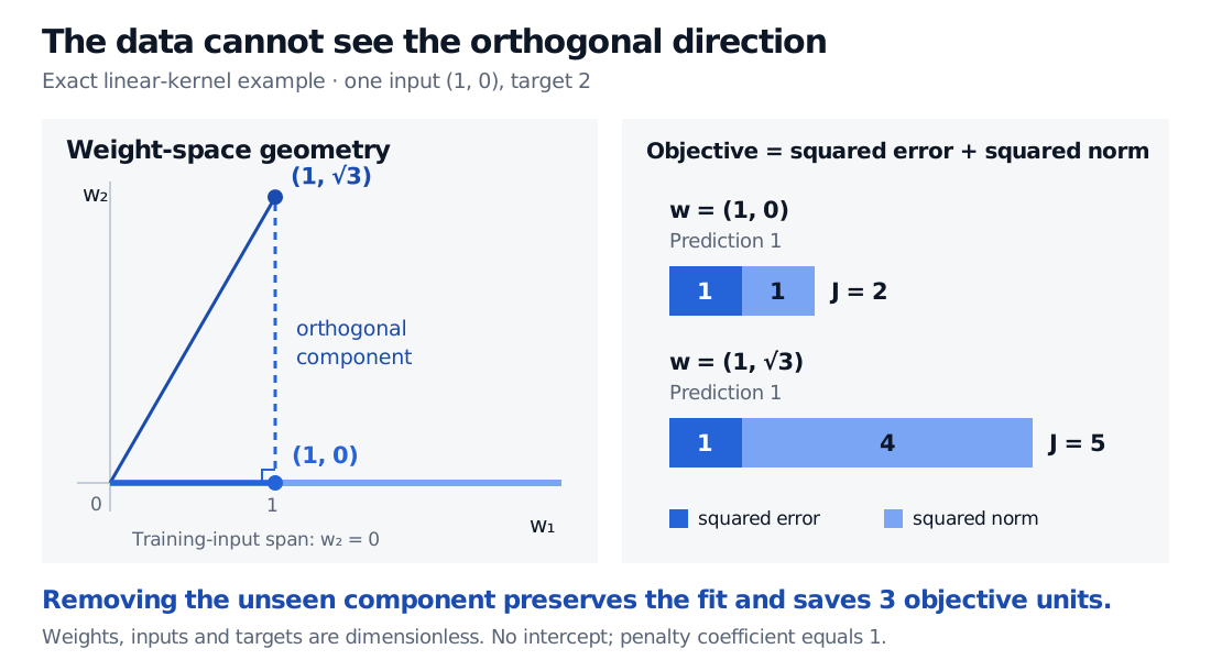
Use the linear kernel $k(x,z)=x^\top z$ on $\mathbb R^2$ . Functions are $f_w(x)=w^\top x$ , with RKHS norm $\lVert f_w\rVert_{\mathcal H}=\lVert w\rVert_2$ . There is one training input $x_1=(1,0)^\top$ , label $y_1=2$ , no intercept and penalty coefficient $1$ . Inputs, targets and weights are dimensionless. The objective is

J(w)=(2-w^\top x_1)^2+\lVert w\rVert_2^2 =(2-w_1)^2+w_1^2+w_2^2 =2(w_1-1)^2+w_2^2+2.

The unique minimum is $w^*=(1,0)^\top$ , with prediction $1$ and objective $2$ . The Hessian is $\operatorname{diag}(4,2)$ , confirming strict convexity. Regularisation deliberately leaves a training residual: the prediction need not equal the label.

Now add $v=(0,\sqrt3)^\top$ , which is orthogonal to the training input. The prediction stays $1$ , but the squared norm rises from $1$ to $4$ . Squared error remains $1$ , so the objective rises from $2$ to $5$ . The extra weight changes predictions at other inputs, yet the objective has no data-fit reason to retain it.

Exact linear-kernel example: weights (1, 0) and (1, square root of 3) both predict 1 at input (1, 0). Their squared errors are both 1, squared norms are 1 and 4, and objectives are 2 and 5.

Original exact example. The vertical component is invisible at the training input and adds 3 objective units; removing it preserves the training prediction.

Finite coefficients, possibly infinite features

The learned

\alpha_i

are scalar coefficients multiplying functions

k(x_i,\cdot)

. They are not coordinates proving that the kernel's feature map has only

n

dimensions. The data select a subspace of dimension at most

n

inside the RKHS; the ambient space may remain infinite-dimensional. This is the bridge from function-space regularisation to a finite kernel method.

Writing

K_{ij}=k(x_i,x_j)

, the Gram matrix gives training predictions

K\alpha

and squared RKHS norm

\alpha^\top K\alpha

. For kernel ridge regression, this yields an objective in

\alpha

using only

K

, labels and the penalty. The representer theorem supplies the form of the solution, not a universal closed-form coefficient formula. Rasmussen and Williams, §6.2

Function uniqueness and coefficient uniqueness are separate. With duplicate centres $x_1=x_2=(1,0)^\top$ , the Gram matrix has every entry equal to $1$ and rank $1$ . Coefficients $(1,0)^\top$ and $(1/2,1/2)^\top$ both represent the same function $f(x)=x^{(1)}$ , where $x^{(1)}$ denotes the input's first coordinate. Their difference lies in the null space of $K$ ; its kernel expansion has zero RKHS norm and is the zero function everywhere, not merely on the sample. A strictly convex function-space objective can therefore have a unique fitted function with nonunique coefficient representations.

Finally, check the model's actual assumptions. A separately unpenalised intercept requires an additional term; a seminorm can leave unpenalised directions. Ordinary neural-network weight decay is not automatically an RKHS norm penalty. The classic result cannot be invoked just because an algorithm uses the word “kernel.” Schölkopf, Herbrich and Smola, Theorem 2; Rasmussen and Williams, §6.2 and its null-space qualification

For the geometry behind the proof, Orthogonal Projections and Minimization Problems develops the perpendicular decomposition and Pythagorean argument (membership required for the full lesson; public preview available).

Sources

Bernhard Schölkopf, Ralf Herbrich and Alex J. Smola, A Generalized Representer Theorem (2001), §2, Theorem 1, its proof and monotonicity remarks; Theorem 2 for an additional parametric component.
Carl Edward Rasmussen and Christopher K. I. Williams, Gaussian Processes for Machine Learning (2006), Chapter 6, §6.1 for the RKHS reproducing property and §6.2 for regularisation and the representer expansion.

The statement needs an objective

Why the unseen directions disappear

An exact two-weight example

Finite coefficients, possibly infinite features

Sources

Related terms

Kernel method and kernel trick

Kernel ridge regression

Orthogonal projection