Use implicit feature inner products to build nonlinear models. An exact quadratic example separates the kernel trick from arbitrary similarity scores and computational promises.
Kernel method and kernel trick
A kernel method learns using inner products in a feature space, represented by a kernel function. The kernel trick evaluates those inner products directly, without constructing the feature vectors. For a quant modelling a nonlinear response to several market indicators, this can introduce interactions without explicitly storing every interaction column.
The starting identity is
k(x,z)=⟨ϕ(x),ϕ(z)⟩.
Here x,z are inputs and ϕ is a feature map. A model linear in ϕ(x) can be nonlinear in x. The trick applies when the learning and prediction rules can be expressed through these inner products; a kernel is not a replacement for arbitrary coordinate operations. Ma and Ng's CS229 notes, §§5.1–5.4, develop this change of representation.
Two routes to 121
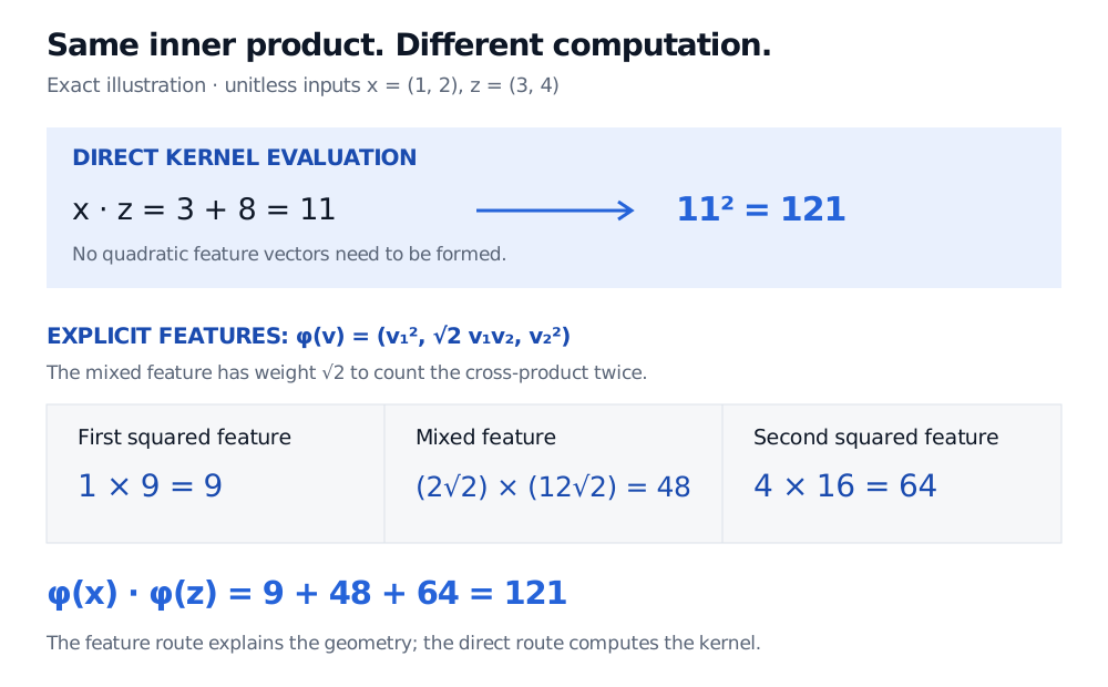
Take the homogeneous quadratic kernel k(x,z)=(x⊤z)2 and fictional, unitless inputs x=(1,2) and z=(3,4). Direct evaluation gives
x⊤z=1⋅3+2⋅4=11,k(x,z)=112=121.
To see the hidden features, choose
ϕ(x)=(x12,2x1x2,x22).
Then ϕ(x)=(1,22,4) and ϕ(z)=(9,122,16). Their inner product is
1⋅9+(22)(122)+4⋅16=9+48+64=121.
The 2 factor matters: squaring a sum includes the mixed product twice. Omitting it would define a different kernel. This particular map contains degree-two terms only, with no constant or linear feature. A linear predictor in these features has the form w1x12+2w2x1x2+w3x22.
Two routes give the same kernel value for unitless inputs x=(1,2) and z=(3,4). The direct route squares the dot product 11 to obtain 121. The explicit-feature route sums three products, 9, 48 and 64, to obtain 121.
Original exact arithmetic. The explicit route reveals which quadratic interactions the direct kernel evaluation includes; it is shown for understanding, not required in a kernel implementation.
This kernel also discards information: ϕ(−x)=ϕ(x). A predictor using only these features cannot distinguish simultaneous sign reversals of all inputs. In a financial application where reversing a signal should reverse its effect, that symmetry could be unsuitable. Choosing a kernel chooses a model's geometry, not merely a computational shortcut.
Similarity needs a mathematical constraint
For the real-valued inner-product kernels discussed here, k must be symmetric and every finite Gram matrix, with entries Kij=k(xi,xj), must be positive semidefinite:
a⊤Ka≥0for every a∈Rn.
This must hold for every finite selection of inputs, not just one dataset. A plausible similarity score need not qualify. GPML §4.1 explains the Gram-matrix condition. The general feature-space existence result and the more specialised spectral expansion are distinguished in Mercer's theorem and valid kernels.
From a kernel to a fitted model
The kernel does not determine the loss or the fitted coefficients. Kernel ridge regression uses squared error with a norm penalty; a kernel support vector machine uses a margin-based classification objective. The same kernel can therefore support different learning problems.
Under the usual regularized RKHS setup, the representer theorem reduces the fitted function to a finite expansion,
f(x)=i=1∑nαik(xi,x),
with a separate intercept if the model specifies one. GPML §§6.1–6.2 connect this form to regularization. The radial basis function kernel offers a different geometry from the quadratic example; its bandwidth controls how quickly similarity decays with distance.
Avoiding explicit features does not remove sample-size costs: storing a dense n-observation Gram matrix requires n2 entries. Kernel choice, input scaling and regularization still affect the fitted model. For a deeper feature-map and Gram-matrix derivation, see the SelfMadeQuant lesson The Kernel Trick (public preview; full lesson requires membership).