Log-linear contingency-table model: Definition & Examples

A log-linear contingency-table model expresses the logarithm of each expected cell count as a sum of category effects and interactions. It lets a quant ask whether two classifications—such as a credit flag and a subsequent payment outcome—occur together more often than their separate frequencies would imply. Its object is the joint count pattern, rather than a continuous return or price series.

The logarithm belongs to the mean

For a two-way table, let $N_{ij}$ be the observed count and $\mu_{ij}=\mathbb{E}[N_{ij}]$ . The usual Poisson formulation is

N_{ij}\sim\operatorname{Poisson}(\mu_{ij}),\qquad \log\mu_{ij}=\lambda+\alpha_i+\beta_j+\gamma_{ij},

with independently sampled Poisson cell counts. The category labels enter as indicator variables; they need not have numerical spacing. This is a generalised linear model with a Poisson distribution and a log link. It does not mean taking

\log N_{ij}

and running ordinary least squares: zero observed counts are legitimate data, and the likelihood models counts directly. Nelder's original formulation makes this mean–data distinction explicit.

If instead the sample contains a fixed total

n

of independent cases, each assigned to exactly one cell, the table is multinomial. Conditioning independent Poisson counts on their total gives that distribution. With a freely fitted total, the two formulations yield the same fitted cell proportions and the same association likelihood-ratio statistic. Fixed-total cell counts themselves are dependent; independence of the sampled cases is the relevant sampling assumption. Evans, §§1–2.

The parameters need constraints. Otherwise one can shift an intercept and compensate through the category effects without changing any fitted mean. Reference-category coding sets the main effects of the reference levels, and every interaction involving a reference level, to zero. Alternative sum-to-zero constraints describe the same model with different coefficient values. Penn State, §10.1.1.

Remove one interaction; change the whole table

Consider 100 fictional independent cases.

A=1

indicates a pre-existing credit flag;

B=1

indicates a later missed payment. These labels establish a chronology, but the table alone does not identify a causal effect.

Classification	$B=0$	$B=1$	Total
$A=0$	30	10	40
$A=1$	10	50	60
Total	40	60	100

With binary indicators $a,b\in\{0,1\}$ , reference coding becomes

\log\mu_{ab}=\lambda+\alpha a+\beta b+\gamma ab.

The saturated model has four free parameters for four cells and reproduces every observed count. Here its maximum-likelihood coefficients are

\lambda=\log30,\qquad \alpha=\beta=\log(1/3),\qquad \gamma=\log15\approx2.70805.

The interaction has a direct interpretation:

\gamma =\log\frac{\mu_{11}\mu_{00}}{\mu_{10}\mu_{01}}.

Thus

e^\gamma

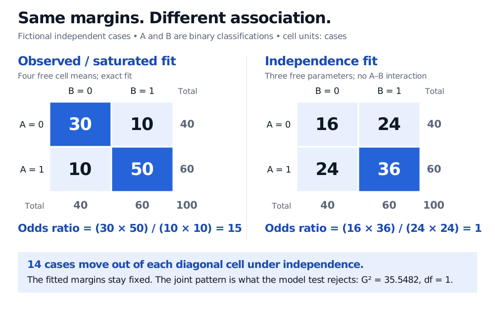
is the odds ratio for

B=1

comparing

A=1

with

A=0

. In this sample it is

(50/10)/(10/30)=15

. This is a ratio of odds, not a fifteenfold probability: the corresponding observed missed-payment fractions are

5/6

and

1/4

Setting $\gamma=0$ imposes independence: the fitted joint probabilities factor into row and column probabilities. The fitted counts become

\widehat\mu_{ij}=\frac{N_{i+}N_{+j}}{n},

so the fitted rows are

(16,24)

and

(24,36)

. Both row totals and both column totals remain unchanged. What disappears is the association: the fitted odds ratio is

1

. Chicago, Chapter 7, slides 3–9.

Fictional observed rows are 30,10 and 10,50; independence-fitted rows are 16,24 and 24,36. Both tables have row and column totals 40 and 60, with total 100. Observed odds ratio 15 becomes fitted odds ratio 1.

The independence fit preserves the margins while lowering each diagonal count by 14 and increasing each off-diagonal count by 14. Counts shown are observed or fitted expected cases, as labelled.

Does independence fit?

The likelihood-ratio test compares independence with the saturated model:

G^2=2\sum_{i,j}N_{ij}\log\frac{N_{ij}}{\widehat\mu_{ij}} \approx35.54818.

For a complete

I\times J

table with positive fitted means and regular estimation, independence uses

I+J-1

free Poisson parameters, compared with

IJ

in the saturated model. Hence the reference degrees of freedom are

(I-1)(J-1)

: here

1

. Penn State, §§10.1.1 and 10.2.6. The asymptotic p-value is about

2.49\times10^{-9}

under the stated sampling model. It is evidence against independence, not a probability that the credit flag causes missed payments. A saturated fit has zero residual deviance by construction; that alone provides no evidence of useful prediction. Evans, §1.1.

A joint model can induce a conditional logistic model. In this binary example,

\log\frac{\mathbb{P}(B=1\mid A=a)}{\mathbb{P}(B=0\mid A=a)} =\log\mu_{a1}-\log\mu_{a0}=\beta+\gamma a.

The shared odds ratio explains the connection. The modelling questions still differ: a log-linear model describes the joint table; logistic regression designates a response and models its conditional probability. Neither construction establishes causality. For larger tables, dropping a three-way interaction permits constant pairwise conditional odds ratios; it does not remove all pairwise association. Chicago, slides 10–11 and 27–35.

Before trusting the statistic

An observed zero can be a sampling zero: an allowed outcome happened not to occur. Its

N\log(N/\widehat\mu)

term is interpreted as zero by a limit. A structural zero is an impossible combination with probability zero. It changes the allowed table, fitting constraints and degrees of freedom; do not insert it into the complete-table formula or repair it with an arbitrary pseudocount. Zero margins or other sparse patterns can put estimates on the boundary and invalidate the usual chi-squared approximation. Penn State, §12.4.

Repeated observations from the same borrower, overlapping horizons and common shocks can invalidate independent-case calibration. Repeated category values across different independent cases are ordinary counts; they are not a separate “ties correction” problem. If categories come from numerical thresholds, declare in advance which interval contains an observation exactly at the boundary. The table only analyses the resulting classification.

For the count likelihood behind this model, Random Variables and Distributions develops Poisson masses and moments. For the nested-model comparison, The Generalized Likelihood Ratio Test derives restricted versus unrestricted likelihood maximisation. Both have public previews; the full lessons require membership.

The logarithm belongs to the mean

Remove one interaction; change the whole table

Does independence fit?

Before trusting the statistic

Sources

Related terms

Generalised linear model

Multinomial distribution

Odds ratio

P-value

Poisson distribution