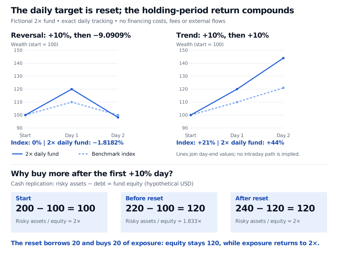
See why daily leverage resets change exposure, why a flat index can leave a 2x fund down, and why a trending path need not produce decay.
Leveraged ETF rebalancing
Leveraged ETF rebalancing is the adjustment of a fund’s benchmark exposure to restore its target leverage relative to its current net assets. For a fund targeting 2× a benchmark’s daily return, that usually means resetting exposure each trading day. The practical consequence is twofold: the fund’s exposure changes as its capital changes, and its holding-period return compounds daily rather than equalling twice the benchmark’s holding-period return.
This is a particular use of rebalancing. The target is an exposure-to-capital ratio, not a fixed number of ETF shares in the investor’s account. Leverage magnifies the day’s return on the capital available that day.
The SEC’s updated investor bulletin of 29 August 2023 explains the daily objective and the potentially substantial divergence over longer periods. Check the particular fund’s stated reset period: a daily target is not a universal feature of every leveraged exchange-traded product.
A flat index can leave the fund below its starting value
Consider a fictional benchmark and an ideal fund that exactly earns twice each daily benchmark return. Start both wealth measures at 100. Assume consecutive close-to-close periods, reinvestment of any distributions, no external flows, zero financing costs, no fees, taxes or trading costs, and successful resets at the day-end prices. These assumptions isolate the reset and compounding mechanism; they do not describe a particular ETF’s realised performance.
Day-end value
Start
After day 1
After day 2
Benchmark wealth
100
110
100
Ideal 2× daily fund wealth
100
120
98.1818
The benchmark rises 10%, then falls 1/11≈9.0909%. Its two-day return is zero because 1.10(10/11)=1. The fund earns +20%, followed by approximately −18.1818%, so
100(1+2×0.10)(1−112)=111080≈98.1818.
Its cumulative return is −1.8182%, despite meeting the daily target exactly. The second day’s loss is applied to 120, not the original 100. This difference is not evidence of failed daily tracking.
For daily benchmark simple returns rt and a constant daily leverage target L, the ideal model is
Rfund=t=1∏T(1+Lrt)−1,Rindex=t=1∏T(1+rt)−1.
In general, Rfund=LRindex. These expressions require positive wealth factors throughout the example. They are not a rule for extending a real fund through a leverage-exhausting loss, contract termination or an inability to rebalance.
The reset buys exposure after a gain
Why change the holdings at all? A simple cash-and-borrowing replication makes the accounting visible. Suppose the fund starts with 100 USD equity, borrows 100 USD at zero interest and buys 200 USD of benchmark assets. After the first +10% day:
Risky assets are worth 220 USD and debt remains 100 USD.
Equity is therefore 120 USD.
Before resetting, asset exposure divided by equity is 220/120≈1.8333, below the 2× target.
Target exposure is 2×120=240 USD. Borrowing another 20 USD and buying 20 USD of assets restores it.
The reset creates no immediate wealth: assets of 240 less debt of 120 still leave 120 USD equity. It changes what is exposed to the next return. On day 2, those assets fall to 240(10/11); subtracting the 120 USD debt leaves 98.1818 USD equity, matching the compound-return calculation.
Fictional costless two-day wealth paths starting at 100. A benchmark round trip ends at 100 while the 2 times daily fund ends at 98.18; two benchmark gains of 10 percent end at index wealth 121 and fund wealth 144. The first gain changes a cash-replicated fund from assets 200, debt 100 and equity 100 to assets 220, debt 100 and equity 120. Buying 20 with new borrowing restores assets 240 divided by equity 120 to 2 times.
Original fictional scenarios. Lines join day-end values, not observed intraday prices. The cash-replication ledger explains exposure changes; actual funds can obtain exposure through derivatives.
More generally, let opening equity be V and opening signed benchmark exposure be LV. In this frictionless linear-exposure model, with no flows or financing charges, a benchmark return r leaves equity V(1+Lr) and existing exposure LV(1+r). The required change in exposure is
ΔX=LV(1+Lr)−LV(1+r)=L(L−1)Vr.
For L>1, the fund increases long exposure after a rise and reduces it after a fall. For L<0, the coefficient is also positive: after a rise, increasing signed exposure means making the short position less negative. The direction follows the benchmark move in both cases, under the stated model. The 2× example gives 2(2−1)(100)(0.10)=20 USD.
Here, “exposure” means economic sensitivity to the benchmark. It is not necessarily a cash purchase of the underlying securities. Funds can use swaps and futures; a change in swap exposure need not appear as an equal-sized purchase by the ETF itself. The Swaps lesson explains how an equity-return leg transfers exposure without transferring ownership of every underlying share. Its public page is a preview; the full lesson is available with free sign-in.
Compounding does not always mean decay
Change the second benchmark return to another +10%, keeping the ideal 2× daily rule. The benchmark gains 1.102−1=21%; the fund gains 1.202−1=44%. That exceeds twice the benchmark’s two-day return, which is 42%.
The reversal and trend examples show why the endpoint alone is insufficient. Daily returns determine compound wealth, and different daily return patterns can give different fund results for the same benchmark holding-period return. A reversal can erode wealth even with perfect tracking; a persistent trend can produce a favourable compounding comparison. “Volatility drag” does not mean a fixed daily charge or a guarantee that every holding period loses money.
This exposure rule also differs from a long-only rebalancing premium example: a leveraged long fund increases exposure after gains to restore its ratio, rather than trimming a winning risky sleeve back to a weight below 100%.
What a quant can infer from the mechanism
The formula provides a conditional exposure estimate, not a complete forecast of closing orders or prices. Applying it to real funds requires current assets, actual exposures, the relevant benchmark move and reset convention. Creations and redemptions, financing, existing hedges and contract terms can change the amount. Counterparties may manage their own hedges, and the fund’s exposure adjustment need not arrive as one visible closing stock order. A mechanical exposure need alone does not establish profitable market impact trading after costs.
For a backtest, compound the daily fund returns or simulate its actual exposure and funding rules. Multiplying a monthly index return by two misses the mechanism. Separate divergence caused by compounding from a failure to meet the daily objective; also separate fund net-asset-value performance from the market-price return earned by someone buying intraday.
The ProShares Ultra QQQ summary prospectus dated 28 September 2026 provides a current concrete example: a 2× daily objective before fees and expenses, daily exposure resetting, derivative use, financing and correlation risks, and different intraday market-price behaviour. It is cited to document the mechanics, not to recommend that fund. Actual results can depart from the ideal equations through costs, imperfect exposure and disrupted rebalancing.
ProShares — Ultra QQQ Summary Prospectus (28 September 2026), “Investment Objective,” “Principal Investment Strategies,” and risks concerning holding periods, correlation and intraday price performance. The examples and cash-replication derivation above are original calculations.
ProShares — Geared ETF FAQs, “Understanding a Daily Investment Objective” and the discussion of fees and embedded financing costs. Read alongside the dated prospectus for the particular fund’s terms.