Distinguish constant-mix excess growth from a return advantage over buy and hold, with a two-period ledger, a trending counterexample and cost limits.
Rebalancing premium
Rebalancing premium is the additional compounded growth attributed to maintaining target portfolio weights as assets move relative to one another. For a quant, its meaning depends on the comparator: growth above the weighted growth of the constituent assets and outperformance of a buy-and-hold portfolio are different quantities. A positive first quantity does not guarantee a positive second one.
Rebalancing restores the allocation; the premium concerns its return consequences. A constant-mix strategy repeatedly restores fixed portfolio weights, while a buy-and-hold strategy lets them drift. The following ledger shows why that difference can help, and why it can also hurt.
Two flat assets, a growing portfolio
Start with one unit of capital, split equally between fictional assets A and B. Assume fractional holdings, reinvested distributions, no external flows, no costs or taxes, and a reset at unchanged prices after the first period. Returns are simple total returns over two equal-length periods; no annualisation is implied. The alternating example is adapted from Willenbrock (2011), §3.
Asset
Period 1
Period 2
Two-period return
A
+25%
−20%
0%
B
−20%
+25%
0%
Each asset ends where it started because 1.25×0.80=1. Buy and hold therefore finishes with the original one unit. The constant-mix portfolio earns
Rp,1=Rp,2=21(25%)+21(−20%)=2.5%,
so its terminal wealth is 1.0252=1.050625: a 5.0625% cumulative return, or 2.5% compounded per period.
The reset is the crucial transaction:
Holding value
After period 1
Trade
After reset
A
0.6250
−0.1125
0.5125
B
0.4000
+0.1125
0.5125
Total
1.0250
0
1.0250
Selling A funds buying B; the reset creates no wealth at execution. It changes the capital exposed to period 2: more is now in B before its recovery. One-way turnover, using pre-trade wealth, is 0.1125/1.025≈10.98%. Counting both purchase and sale gives approximately 21.95% gross traded value relative to wealth. Neither percentage is a fee rate.
Change the second period and buy and hold wins
Keep the first period unchanged. Now let A rise 25% again and B fall 20% again. Resetting to 50/50 still earns 2.5% in each period, so constant mix again finishes at 1.050625. But buy and hold finishes at
21(1.25)2+21(0.80)2=1.10125,
a 10.125% cumulative return. The initial A holding grows into a larger portfolio weight, and its second gain benefits more capital. Rebalancing sold part of that continuing winner.
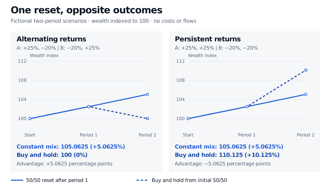
Fictional wealth indexed to 100. With alternating returns, 50/50 constant mix ends at 105.0625 and buy and hold at 100. With persistent returns, constant mix again ends at 105.0625 but buy and hold reaches 110.125.
Original endpoint comparison with one costless 50/50 reset after period 1. The alternating scenario is adapted from Willenbrock (2011), §3; the persistent-return counterexample changes the second period. Connecting segments show period endpoints, not observed intraperiod prices.
The constant-mix advantage against buy and hold changes from +5.0625 to −5.0625 percentage points. This is a change in the supplied return path, not a different rebalancing rule. Neither scenario estimates expected alpha. Bernstein’s “Rebalancing: Practical Issues” likewise distinguishes a return increment above averaged asset growth from an actual comparison with an unrebalanced portfolio.
What “excess growth” measures
There is an exact finite-period log-growth identity behind the intuition. For fixed nonnegative weights wi summing to one and asset returns ri,t>−1, define
Δt=log(i∑wi(1+ri,t))−i∑wilog(1+ri,t)≥0.
The inequality follows from concavity of the logarithm. Summing over periods gives the constant-mix portfolio’s total log return minus the fixed-weight average of the assets’ total log returns. That reference is a weighted geometric basket of asset wealth relatives. It is not the wealth of the buy-and-hold portfolio, which is the weighted arithmetic sum of those wealth relatives. The persistent-return counterexample can therefore have positive log-growth gaps while constant mix underperforms buy and hold.
In a frictionless continuous-path diffusion model, Fernholz and Karatzas, equations (1.12)–(1.13), express the corresponding instantaneous log-growth drift as
Here γi is asset i’s instantaneous log-growth drift, and aij is its instantaneous covariance rate with asset j. The second sum is portfolio variance per unit time. The excess growth rateγp∗ is nonnegative for long-only weights; it can be zero when the assets have identical return shocks. It compares portfolio log growth with weighted asset log growth, and is not risk-free excess return or guaranteed benchmark outperformance.
This diffusion identity is exact within its model. Replacing its variance rates with sample variances of finite-period simple returns gives an approximation, not an exact backtest decomposition. Lower correlation, holding asset volatilities and weights fixed, can enlarge the excess-growth term; it does not settle the buy-and-hold comparison.
The premium must survive implementation
A usable claim states the assets, starting weights, horizon, reset schedule, return convention, comparator and cost basis. Persistent relative trends can favour drifting weights; reversals can favour the reset. Changing the rebalance frequency changes the trades and the return path sampled. More frequent trading does not establish a larger net premium.
Spreads, commissions, market impact and realised taxes can consume a gross benefit. Costs paid from the portfolio also reduce the capital available for subsequent returns, so the costless ledger cannot simply be treated as a net result. Transaction Costs and Implementation develops linear costs and no-trade regions; its public page is a preview and the full lesson requires membership. The relevant decision is whether restoring the chosen exposure justifies the trades under those constraints, rather than assuming that every reset earns a bonus.
William J. Bernstein — Rebalancing: Practical Issues (1997), “When It Doesn’t Work” and the closing frequency/cost discussion: the comparator, allocation drift and implementation trade-offs. Its historical tax rates and backtest returns are not used as current assumptions here.