Jump risk exposes a position to a price gap before it can rebalance. Separate Poisson event counts from jump probabilities, and see why a diffusion delta and a stop trigger do not remove the gap.
Jump risk
Jump risk is exposure to a sudden discontinuous change in an asset’s price: the price can move from one level to another without passing through every intermediate level. A position that looks well hedged against small moves can suffer a loss before its holder can rebalance. The same gap can carry a price through a stop level without providing an execution at that level.
Jumps can be upward or downward. An earnings announcement, default or policy surprise can change value abruptly; a known announcement date still leaves the size and direction uncertain. An overnight gap is also a trading problem because the investor may have had no opportunity to transact while the market was closed. A gap between sampled observations alone does not prove a mathematical discontinuity: a continuous price could have moved rapidly between observations.
Separate arrival frequency from jump size
A Poisson process models event arrivals, not the price impact by itself. Its intensity λ is an expected count per unit time. Jump risk also needs a rule for the size and direction of each price change. Constant Poisson intensity and independent arrivals are simplifying assumptions; they need not describe scheduled announcements or clustered shocks.
Consider this synthetic pricing model, with time t in years and prices in currency units per share:
St=100e0.02t(0.9)Nt,Nt∼Poisson(0.2t).
The entire process N is stipulated to have independent, stationary Poisson increments under the risk-neutral measure Q. Interest, dividends and trading costs are zero, and there is no Brownian component. Between jumps the price grows continuously at rate 0.02 per year. Each jump cuts the immediately preceding price by 10%.
Over one year, the exact Poisson law gives:
Jump count N1
Probability under the stipulated Q
Terminal price S1
Zero
81.8731%
102.02
Exactly one
16.3746%
91.82
Two or more
1.7523%
At most 82.64
Prices and percentages are rounded. The last row groups every count from two upward; 82.64 is the rounded price with exactly two jumps. Repeated jumps multiply: two 10% cuts leave a factor 0.92=0.81, before allowing for the continuous growth.
An expected count of 0.2 is not a 20% probability of a jump. Here,
Q(N1≥1)=1−e−0.2≈18.1269%.
These probabilities are chosen pricing inputs, not forecasts of how often real prices will jump. For the count law and its distinction from an arrival rate, Random Variables and Distributions develops Poisson masses and moments; the full lesson requires membership and has a public preview.
Why the price grows between downward jumps
The continuous growth compensates for the expected downward jump contribution. The Poisson generating function gives
EQ[St]=100e0.02texp(0.2t(0.9−1))=100.
Independent increments give the corresponding conditional martingale property. This is consistent with the model’s zero interest rate and zero dividends. The between-jump growth is not interest earned without risk: a jump can interrupt it. An expected price of 100 does not guarantee a terminal price of 100.
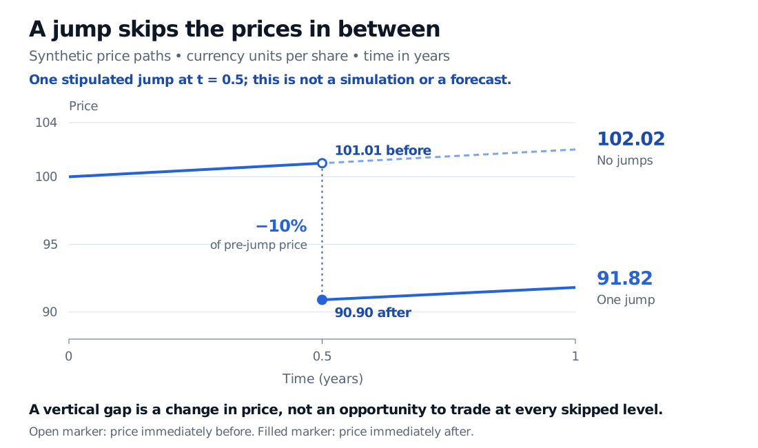
Synthetic price path starting at 100: a stipulated jump at year 0.5 takes price from 101.01 immediately before to 90.90 immediately after, a 10% fall. The one-jump path ends at 91.82; the dashed zero-jump path ends at 102.02.
Original synthetic illustration of the stated pricing law. The jump time is chosen for illustration, not randomly sampled. Open and filled markers distinguish the price immediately before and after the jump; the vertical dotted segment does not represent trades at intermediate prices.
A diffusion delta is a local hedge
An option’s delta describes its local sensitivity to the underlying price. For an option value C(t,S), the usual diffusion hedge uses Δ=∂C/∂S. But a finite jump from S to S(1+j) changes the option value by
C(t,S(1+j))−C(t,S),
while Δ shares change in value by ΔSj. Thus the instantaneous change of a long option hedged with Δ short shares is
C(t,S(1+j))−C(t,S)−ΔSj.
That expression need not vanish. A derivative is a local slope, whereas the price gap requires a finite difference. A small-move approximation using gamma can describe curvature locally; it is not an exact identity for an arbitrary jump. Trading more frequently does not supply an execution inside an instantaneous gap. Merton’s original jump-diffusion paper makes this distinction between continuous and jump exposures.
This does not mean every model with jumps rules out replication. In the special fixed-size pure Poisson model used above, a finite-jump hedge can permit exact replication under ideal trading assumptions. Its hedge ratio need not be the diffusion delta. With uncertain jump sizes or both diffusion and jump shocks, the available assets may not span every source of risk. The hedge’s instruments and model matter.
A stop trigger is not a price floor
A conventional stop order becomes a market order when triggered. In U.S. stock-market guidance, the SEC explains that execution can differ substantially from the stop price, depending on available liquidity. A stop-limit order adds a price constraint but can remain unexecuted. Trigger rules also vary by venue and broker. These are execution conditions, not a mechanism that makes a price path continuous. See the SEC’s stop-order bulletin.
For risk management, test the jump scenario and the trade response together: the size and sign of the shock, whether several positions jump together, which hedges still pay, and where trading can resume. A quiet historical sample or a delta-neutral starting position does not settle those questions. Pricing probabilities under Q also do not replace estimates and stress scenarios for real-world losses.
Sources
Robert C. Merton, “Option Pricing When Underlying Stock Returns Are Discontinuous”, Journal of Financial Economics 3 (1976), pp. 125–144, especially pp. 128–132 and footnote 9: multiplicative Poisson jumps, finite hedge residuals and the fixed-size pure Poisson exception.
Rama Cont and Peter Tankov, Financial Modelling with Jump Processes, Chapman & Hall/CRC, 2004, §§2.5.2–2.5.4 and §10.4.2, pp. 337–338: Poisson counts, compensation and the distinction between a diffusion delta and a finite-jump hedge.