Implicit differentiation: Definition & Examples

Implicit differentiation finds a derivative from an equation relating variables, without first isolating the dependent variable. If an equation ties two exposures together, it tells you how one must adjust when the other changes while the equation remains satisfied.

The essential step is to write

y=y(x)

mentally, even when the equation leaves that dependence hidden. Differentiating

y^2

with respect to

x

gives

2y\,dy/dx

, not

2y

. That extra factor is the chain rule, and it is what turns the equation into a sensitivity calculation.

Trading one exposure against another

Suppose a risk manager stipulates a hypothetical budget for two nonnegative, dimensionless normalized exposures:

x^2+y^2=100,\qquad x\ge0,\quad y\ge0.

This is a chosen quadratic constraint, not a universal portfolio or value-at-risk rule. Actual risk aggregation depends on the model, including dependence between positions. Here the question is deliberately narrower: along this fixed budget, how much must $y$ change when $x$ increases?

Differentiate the whole equation with respect to $x$ :

2x+2y\frac{dy}{dx}=0, \qquad \frac{dy}{dx}=-\frac{x}{y},\quad y\ne0.

At $x=6$ , the nonnegative solution is $y=8$ , because $6^2+8^2=100$ . Therefore

\left.\frac{dy}{dx}\right|_{(6,8)}=-\frac68=-0.75.

Locally, increasing $x$ by one normalized unit requires a reduction of about $0.75$ normalized units in $y$ . This is a marginal exchange rate along the constraint; it does not say that a full one-unit move has exactly that effect.

For a smaller move from $x=6$ to $6.1$ , the tangent estimate is

y\approx8-0.75(0.1)=7.925.

Re-solving the constraint gives $y=\sqrt{100-6.1^2}\approx7.924014$ . The tangent estimate is about $0.000986$ too high. A derivative supplies a local approximation; an exact finite adjustment must still satisfy the original equation.

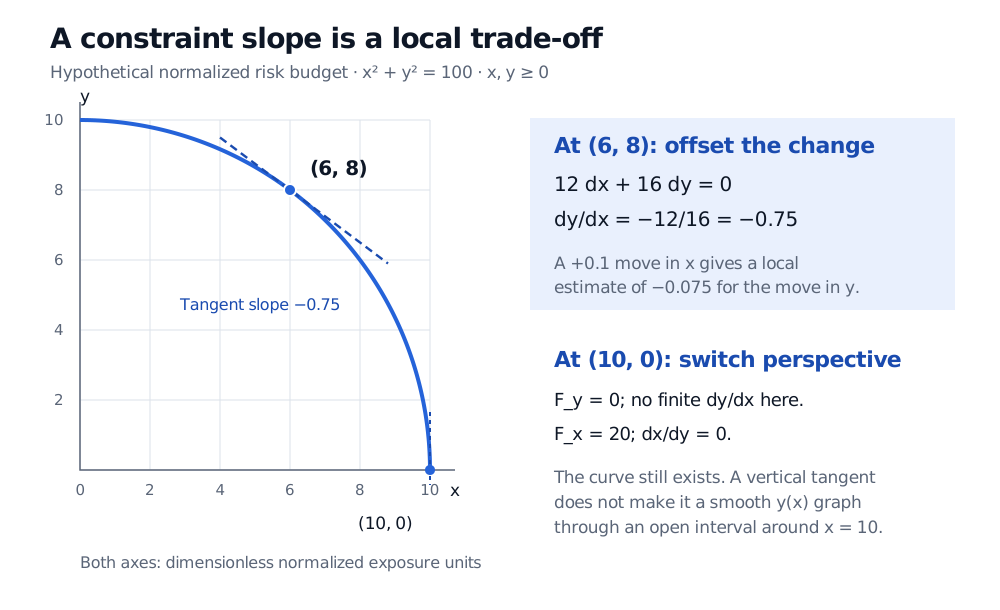
Nonnegative first-quadrant constraint x squared plus y squared equals 100, in dimensionless normalized exposure units. At 6,8 the tangent slope is minus 0.75. At the boundary point 10,0 the tangent is vertical: dy/dx is not finite, although dx/dy is zero.

Original hypothetical normalized-exposure model. The blue curve satisfies the budget; the dashed line at (6, 8) is its local tangent. The vertical tangent at the boundary (10, 0) shows why the denominator matters.

The compact formula, and what it holds fixed

Write a general relation as $F(x,y)=0$ . Along a differentiable solution branch $y(x)$ , the multivariable chain rule gives

\frac{d}{dx}F(x,y(x)) =F_x+F_y\frac{dy}{dx}=0.

Here

F_x

and

F_y

are partial derivatives: each differentiates

F

while holding its other input fixed. Solving gives

\boxed{\frac{dy}{dx}=-\frac{F_x}{F_y}},\qquad F_y\ne0,

with both partial derivatives evaluated at the same point on the chosen branch. In the budget example, $F=x^2+y^2-100$ , so $F_x=2x$ and $F_y=2y$ .

There is a useful balance interpretation: $F_x\,dx+F_y\,dy=0$ says the first-order effect of changing $x$ is offset by the first-order effect of adjusting $y$ . A small absolute $F_y$ can make the adjustment large, provided $F_x$ does not vanish too. The inputs' units and scaling matter when comparing such slopes across models.

If the budget itself changes, the right side no longer has zero derivative. For $x^2+y^2=B(x)$ , the equation becomes $2x+2y\,dy/dx=B'(x)$ . Always identify what remains fixed before interpreting the answer.

A slope belongs to a branch

The unrestricted circle equation permits $y=\pm\sqrt{100-x^2}$ . It does not specify one global $y(x)$ : for most admissible $x$ there are two possible values. Our nonnegative-exposure restriction selects the upper branch for $0\le x\le10$ , with $y>0$ in its interior. Explicit differentiation of that branch gives

\frac{d}{dx}\sqrt{100-x^2} =-\frac{x}{\sqrt{100-x^2}},

which agrees with the implicit calculation. Choosing a branch and its domain is separate from differentiating it; neither operation automatically establishes a global inverse function.

The implicit function theorem supplies a standard local guarantee: if

F

has continuous first partial derivatives near a solution

(a,b)

and

F_y(a,b)\ne0

, the equation has a unique continuously differentiable branch

y(x)

near that point, with values near

b

. This is a neighbourhood result, not a promise about every solution of the equation. MIT's course notes explain the distinction between calculating a branch's derivative and establishing that the branch exists.

At the budget's boundary

(10,0)

F_y=0

. The positive branch's slope tends to

-\infty

x

approaches 10 from below; there is no finite $dy/dx$ there. The circle has a vertical tangent. Switching coordinates works locally for the unrestricted circle:

F_x=20\ne0

, so

dx/dy=-F_y/F_x=0

. The exposure model retains only the nonnegative portion of that curve.

Failure of

F_y\ne0

does not always mean a differentiable branch is absent. For example,

(y-x)^3=0

defines the smooth branch

y=x

, yet both first partial derivatives vanish along it. The ratio formula becomes

0/0

because this representation is degenerate. Simplifying the equation reveals the branch. Check the equation and geometry instead of treating a failed sufficient condition as a proof of nonexistence.

For more worked differentiation, the Library's Implicit Differentiation and Logarithmic Derivatives develops the mathematical method using circles and the folium of Descartes. The public page is a preview; the full lesson requires membership.

Sources

James Stewart, Single Variable Calculus: Early Transcendentals, 6th edition, Thomson Brooks/Cole, 2008, §3.5, especially the dependent-variable chain rule and explicit checks for different branches.
MIT World Web Math, “Implicit Differentiation” — differentiating relations and identifying upper and lower circle branches.
MIT OpenCourseWare, 18.024 Calculus with Theory, Chapter C, “Implicit differentiation,” PDF pp. 14–18 — local existence conditions, branch selection and coordinate choice.

Trading one exposure against another

The compact formula, and what it holds fixed

A slope belongs to a branch

Sources

Related terms

Chain rule

Constraint

Derivative (calculus)

Inverse function

Partial derivative