The imaginary unit satisfies i² = −1. See why multiplying by i turns a vector through 90 degrees, how its powers cycle, and where complex weights enter finance.
Imaginary unit
The imaginary unit, written i, is the complex number defined by i2=−1. No real number has this property: the square of every real number is nonnegative. Introducing i extends real arithmetic to complex numbers, written a+bi with real a and b.
The word “imaginary” does not mean an error or an unobservable cash balance. It names a number that lets us work with two coordinates using ordinary addition and multiplication. In quantitative finance, i appears in frequency analysis and transform methods for option valuation; the returns being analysed and the final cash prices remain real.
The rule that does the work
Expand brackets as usual and replace every i2 by −1. For example,
i(3+4i)=3i+4i2=−4+3i.
It is the 4i2 term that moves into the real coordinate with a negative sign. Multiplying by i does not simply attach an i to each coordinate.
The powers repeat every four steps:
Power
Value
Action on a nonzero complex number
i0
1
No turn
i1
i
Counterclockwise quarter-turn
i2
−1
Half-turn
i3
−i
Counterclockwise three-quarter-turn
i4
1
One complete turn
Consequently, i10=i8i2=−1. Also, 1/i=−i, since i(−i)=1. Dividing by i therefore makes a clockwise quarter-turn.
A quarter-turn, not a change in size
On the complex plane, the real coordinate is horizontal and the imaginary coordinate is vertical. In general,
i(a+bi)=−b+ai,(a,b)⟼(−b,a).
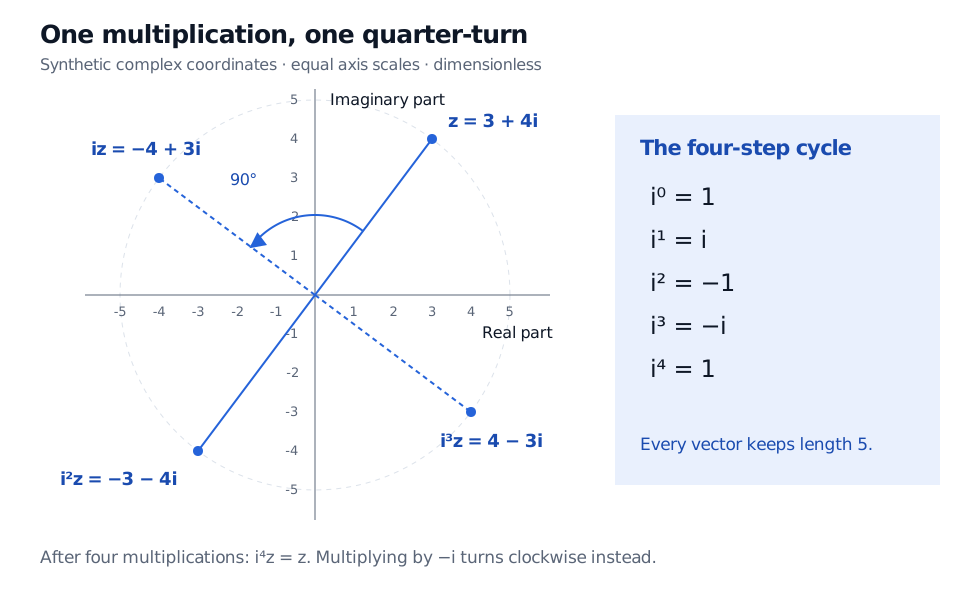
The new coordinates have the same squared length: (−b)2+a2=a2+b2. Thus multiplication by i preserves the complex modulus. Starting from z=3+4i, whose modulus is 5, successive multiplications give
3+4i⟶−4+3i⟶−3−4i⟶4−3i⟶3+4i.
Four counterclockwise quarter-turns carry 3 plus 4i to minus 4 plus 3i, minus 3 minus 4i, 4 minus 3i, then back to the start. All four vectors have dimensionless length 5.
Original dimensionless example. Each multiplication by i rotates the vector through 90 degrees while preserving its length; four restore the original point.
This is a different operation from taking a complex conjugate: conjugation sends a+bi to a−bi, reflecting across the real axis. For our example the conjugate is 3−4i, whereas iz=−4+3i.
Suppose an analyst has four synthetic, equally spaced daily returns, in decimal units:
r0=0.01,r1=0,r2=−0.01,r3=0.
A Fourier transform compares data with oscillations. For this four-observation example, define the unnormalised forward discrete transform by
Rk=n=0∑3rne−2πikn/4,k=0,1,2,3.
At k=1, the weights are 1,−i,−1,i: clockwise quarter-turns because the exponent has a minus sign. Therefore
R1=0.01(1)+0(−i)+(−0.01)(−1)+0(i)=0.02.
The complex weights extract the strength and phase of a sampled oscillation. The value 0.02 is a transform coefficient under the stated normalisation, not a 2% cumulative return, an annualised statistic or a trading forecast. Different sign and scaling conventions must be tracked when comparing software. Four constructed observations offer no evidence that a market cycle exists or will persist.
Option-pricing methods use related complex exponentials inside characteristic functions, which encode a probability distribution. Carr and Madan's FFT valuation method uses a risk-neutral transform to recover option values. The imaginary coordinate belongs to the calculation, not to the currency denomination of the option price.
For that financial extension, Fourier Transform Pricing, §§7.2–7.4 connects complex exponentials to characteristic functions, inversion and the discrete transform. Its public page provides a preview; the full lesson requires membership.
Be careful with square roots
Both i and −i solve w2=−1. The notation −1=i selects the principal square root; it does not say the quadratic equation has only one solution.
The familiar real-number rule ab=ab cannot be extended indiscriminately to complex principal roots. Setting a=b=−1 demonstrates the failure:
−1−1=i2=−1,(−1)(−1)=1=1.
Defining i through i2=−1 keeps the algebra clear. When a financial model later introduces complex square roots or logarithms, its branch conventions must also be respected.
Sources
Sheldon Axler, Linear Algebra Done Right, 2nd edition, Chapter 1, “Complex Numbers,” pp. 2–3 — construction of complex arithmetic and the identity i2=−1.