The Hodrick–Prescott (HP) filter decomposes a time series into a smooth trend and a residual by penalising changes in the trend’s slope. It gives a quant a reproducible way to describe departures from a chosen smooth path. The fitted historical trend usually uses later observations, so treating a retrospective HP chart as a contemporaneous signal can contaminate a trading backtest.
What “smooth” costs
Let be equally spaced, finite observations, with . In the finite-sample version used here, choose and solve
The first sum charges for missing the observations. The second charges for changing the slope: is the change between two successive first differences. A straight, steeply rising line has zero curvature penalty; “smooth” does not mean “flat”. This is the fit-versus-smoothness trade-off in Hodrick and Prescott’s decomposition procedure.
The boundary convention matters. Here every observation has unit weight, only the second differences entirely inside the sample are penalised, and there are no padded observations or imposed endpoint slopes. The endpoints are estimated jointly with the interior; they are not fixed to the first and last data values.
If maps a vector to those second differences, the first-order conditions give
The inverse expresses the mathematics; a numerical implementation can solve the linear system directly. For nonnegative , the identity term makes the system positive definite and the solution unique. The residual is conventionally called the cycle, but that label alone identifies neither an economic mechanism nor a recurring period.
A five-point pulse, then a revised history
Take the fictional observations 0, 0, 10, 0, 0 index points and set solely to make the arithmetic transparent. The three rows of place coefficients on periods 1–3, 2–4 and 3–5 respectively. Solving gives
Only 4.167 of the central observation’s 10 points goes into the fitted trend. The residual at that date is 5.833 points; the zero observations around it have negative residuals because their fitted trends are positive. This is the stated optimisation allocating a pulse between its two components, not evidence that the fictional series has an economic boom and bust.
Now stand at period 4, when the fifth observation is unavailable. With the same and boundary rule, the four-point fit is
Its last value is 3.030. Appending period 5’s zero changes the estimate for period 4 to 2.500, a revision of points. None of the first four observations changed.
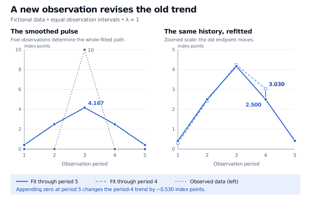
The full-sample fit smooths the pulse; the zoomed panel reveals a historical revision caused only by extending the sample. The two panels use different vertical scales.
The ordinary full-sample filter is two-sided: an interior trend estimate generally depends on observations on both sides of its date. Near a boundary, the available observations are asymmetric and the effective weights differ. Hamilton’s analysis, §§2–3.2, explains why endpoint estimates and retrospective interior estimates can tell different stories.
Using the five-point period-4 estimate in a decision supposedly made at period 4 introduces look-ahead bias. An expanding-sample implementation can instead fit only the observations available at each decision and retain that fit’s endpoint. It must also preserve the data vintage and choose its parameters using information available then. That produces a different sequence from taking an interior column of the final fit. It removes this particular future-observation leak, while leaving the question of whether the chosen decomposition is economically useful.
The Point-in-Time Data lesson develops transformation cutoffs, historical versions and truncation checks. Its preview is public; the full lesson requires membership.
What changing can—and cannot—settle
At , the trend equals the data and the residual is zero. As grows, changes in slope become more expensive. In the limit , the trend approaches the least-squares straight line through the sample. For our symmetric pulse, that limiting line is the constant 2 index points. Finite positive allows curvature; it does not specify a forecast horizon.
The familiar quarterly macroeconomic convention is a historical modelling choice, not a general calibration for prices or trading signals. Ravn and Uhlig study how an existing choice can be adjusted when observation frequency changes. Their fourth-power rule aims to approximately preserve the filter’s frequency response; it does not establish that the starting parameter or the HP decomposition is appropriate for a particular dataset. Their time-domain analysis also distinguishes time aggregation from point sampling.
Finally, an apparently oscillating residual is insufficient evidence for a tradable economic cycle. Hamilton shows how HP filtering can create dynamic patterns from a random walk. Nor does a smooth fitted path establish stationarity. A quant using this decomposition should state its economic purpose, sample boundaries, parameter and information cutoff before interpreting the resulting “cycle”.
Sources
- Hodrick, R. J., and Prescott, E. C. (1997), Postwar U.S. Business Cycles: An Empirical Investigation, §1: squared second-difference smoothing and the linear-trend limit.
- Ravn, M. O., and Uhlig, H. (2002), On Adjusting the Hodrick-Prescott Filter for the Frequency of Observations, §§II–III: time aggregation, point sampling and approximate frequency-response matching.
- Hamilton, J. D., Why You Should Never Use the Hodrick-Prescott Filter, author’s May 2017 revised paper, §§2–3; published in The Review of Economics and Statistics in 2018. The finite-sample pulse, exact solutions and figure above are original illustrations.