The historical November–April stock-return pattern, why stronger winter returns need not make a cash-switching strategy win, and how to test the calendar rule.
Halloween effect
The Halloween effect is the historical stock-return pattern in which November through April has a higher average return than May through October. It is a particular form of seasonality, associated with the saying “sell in May and go away.” For a quant, its first use is as a calendar hypothesis to test. Turning it into a switching strategy requires a second comparison: the return on equities forgone from May through October versus the return earned on cash over those same months.
“Winter” and “summer” in this literature are shorthand for those Northern Hemisphere calendar windows. They do not change places for an Australian market test. Neither the name nor the historical pattern establishes that a particular coming November–April will outperform.
Two claims that sound alike
A seasonal-return claim says that the two equity windows have different means. A strategy claim says that holding equities for one window and cash for the other improves an investor's result. The first does not imply the second.
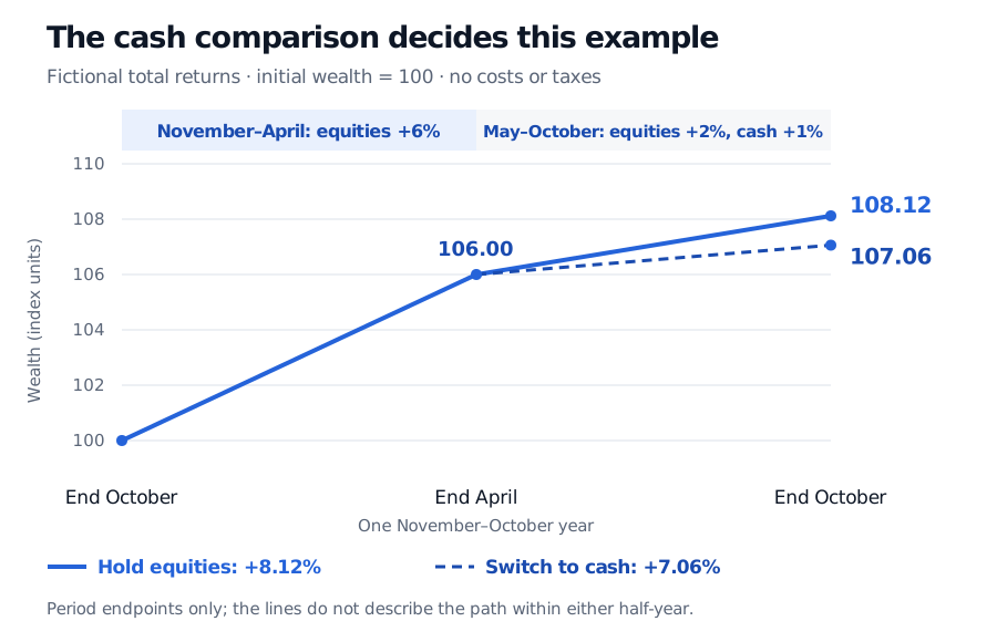
Consider one fictional November–October year, measured in a single currency. Start with wealth of 100 immediately before November. Assume an investable equity portfolio earns a 6% total return over November–April and 2% over May–October. A specified cash investment earns 1% over May–October. These are realised six-month simple returns, including reinvested income where applicable; they are not annualised rates or estimates from market data. Ignore fees, taxes and trading costs for this calculation.
Position during May–October
Wealth after November–April
Wealth at the following October end
Full-year return
Keep holding equities
106.00
108.12
8.12%
Switch the entire portfolio into cash
106.00
107.06
7.06%
The equity windows display the named ordering: 6% exceeds 2%. Yet switching loses 1.06 percentage points of full-year return because the cash investment earns less than the equities it replaces.
Writing the three six-month returns as RW, RS and RC:
In this costless, fully invested comparison, their difference is
Rswitch−Rhold=(1+RW)(RC−RS).
Provided wealth after the first window is positive, it is the cash-versus-equity return in the second window, rather than the winter-versus-summer equity gap, that determines the sign. Lower equity exposure could change portfolio risk as well; the wealth calculation alone says nothing about volatility, drawdowns or risk-adjusted performance.
Fictional wealth starts at 100 and reaches 106 after November–April. Holding equities through May–October ends at 108.12; switching to cash ends at 107.06, a 1.06-point wealth shortfall.
Original fictional example. Lines connect the three period endpoints, not an observed or simulated path within each half-year; costs and taxes are excluded.
Multiplying wealth factors also prevents a second mistake. Adding 6% and 2% gives 8%, missing the return on the first window's gains. Annualising the separate half-year returns and adding them would be a different error: both describe rates over hypothetical full years, not two adjacent pieces of this realised year. For multiple years, compound the actual sequence; a pair of average seasonal returns does not reproduce that sequence's terminal wealth.
What the research establishes—and what remains disputed
Bouman and Jacobsen's 2002 paper reported the November–April ordering in 36 of 37 markets studied. That is a historical cross-market finding, not a statement that every country result was individually significant or that the rule wins every year. Their abstract also reports no convincing explanation for the puzzle. Original paper and abstract.
Later research does not deliver one uncontested implementation verdict. In a working paper hosted by TIAS, Jacobsen and Zhang report broad supporting evidence; Table 3 labels its out-of-sample calendar-effect comparison September 1998–July 2011. Its introduction explicitly distinguishes a winter–summer difference from testing summer equity returns against short-term interest rates. Jacobsen and Zhang, introduction and out-of-sample discussion.
Dichtl and Drobetz's April 2014 working paper instead stresses investable instruments, reinvested dividends, costs and the period after the 2002 journal publication. It finds weaker evidence in those narrower samples, including 2003–2012. These are different sample and implementation designs, not a single experiment repeated with identical inputs. Dichtl and Drobetz, §§3–5.
The distinction matters: a long price-index history can help investigate a calendar pattern, while an investor needs an available instrument's total return. A cash-switching investor misses the equity dividends paid during the absent months. A price-only comparison can therefore misstate the relative wealth outcome.
Specify the calendar before testing it
A reproducible backtest needs an executable rule, not just six month names. Define entry and exit at a particular local-market close or next open, including what happens when month end is not a trading day. November's monthly close-to-close return includes the movement from the preceding October close: buying only after a subsequent opening does not capture exactly the same interval.
Then fix the market, currency, sample start and end, dividend convention, cash instrument and its realised return. For futures, document the contract series, rolls, collateral return and financing treatment; a futures price series alone is not the wealth of a fully collateralised equity-and-cash strategy. Charge spreads, fees, slippage and any relevant taxes to the actual switches. These transaction costs reduce the switching result relative to its frictionless counterpart.
Searching across countries, alternative month boundaries and sample endpoints until one split looks strong introduces data snooping. Preserve an untouched evaluation period and disclose how many variants were tried. Outlier sensitivity and uncertainty matter too: markets share shocks, so a positive result in many countries is not equivalent to as many independent confirmations.
Finally, distinguish the six-month pattern from the January effect, which may contribute to the November–April average. Controlling for January asks whether evidence remains beyond that month. It still does not establish that vacations, daylight or any other seasonal story causes returns. A calendar indicator is a predictor label; causality requires additional evidence.
For the implementation layer, Transaction Costs and Implementation develops spread, impact and cost-aware trading models. The public preview is open; the full lesson requires membership.