The historical small-stock January return pattern, why tax-loss selling is only a partial explanation, and how compounding, trading windows and costs change its interpretation.
January effect
The January effect is the historical tendency for stock returns to be unusually high in January, especially among small-capitalisation stocks and near the first trading days of the year. For a quant, it is a question about when a return premium occurs: an annual small-stock result can be driven disproportionately by one short calendar window. It is a particular calendar anomaly, not a guarantee that January will be positive or that small stocks will beat large stocks every January.
The term also differs from the January barometer, the claim that January's market direction predicts the rest of the year. A high average January return does not establish that forecasting relationship.
What the historical finding actually says
Rozeff and Kinney (1976) studied NYSE monthly returns over 1904–1974. Their abstract reports differences in average returns across months, mainly attributable to January, with the 1929–1940 subperiod an exception to statistical significance. That is evidence about a sample and its subperiods, rather than a permanent feature of every stock market.
Keim (1983) sharpened the small-stock connection using NYSE and AMEX stocks over 1963–1979: roughly half the average size effect in that sample came from January abnormal returns, and more than half the January premium came from the first trading week. A full-month average can therefore hide a much narrower turn-of-year concentration.
Those are different comparisons. “January versus other months” measures seasonality within a portfolio. “Small versus large in January” measures a cross-sectional spread during January. A benchmark comparison is not automatically risk-adjusted alpha; small stocks can have different risk exposures and liquidity from the benchmark. State which return, universe and comparison a claimed January effect uses.
A January gap does not occur twelve times
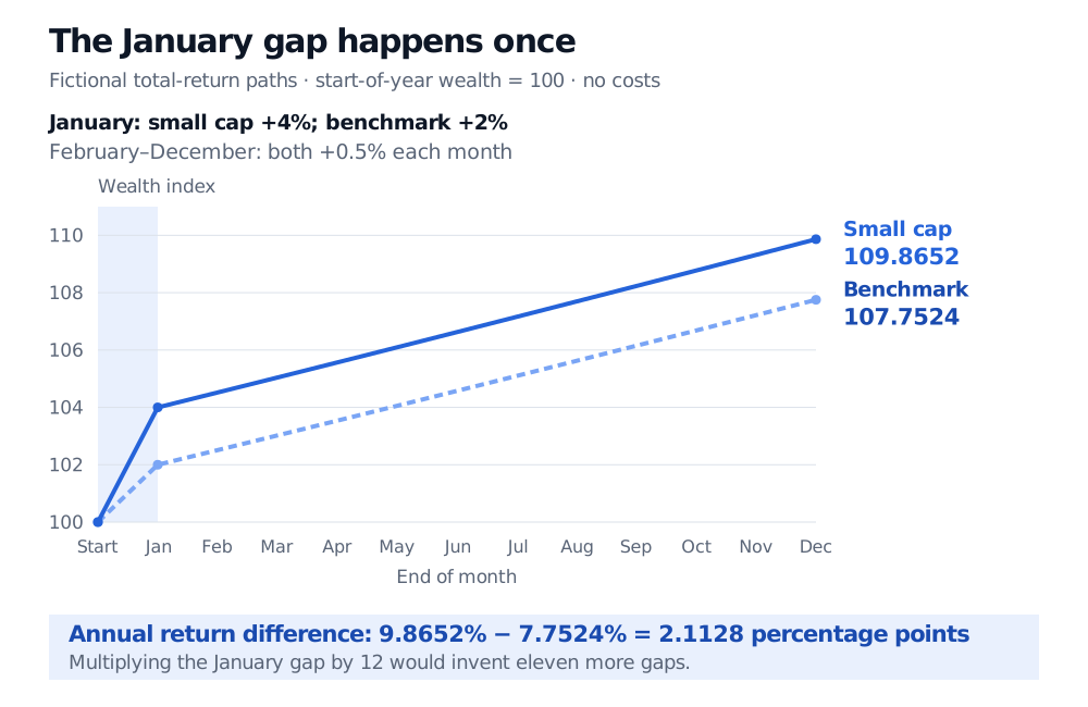
Consider two fictional, fully invested portfolios with reinvested total returns, no cash flows and no trading costs. Both start the year at a wealth index of 100. The small-cap portfolio earns 4% in January and the benchmark earns 2%. Each then earns 0.5% per month from February through December.
The January difference is 2 percentage points. The full-year simple returns compound as
Fictional wealth paths start at 100, reach 104 and 102 after January, then both grow 0.5% monthly. December wealth is 109.8652 and 107.7524; annual returns differ by 2.1128 percentage points.
Original fictional compounding example. The January gap occurs once; subsequent identical percentage returns grow both wealth levels. Lines connect month-end observations, not observed market prices.
Multiplying the January gap by twelve would give 24 percentage points and assume eleven additional gaps that the example explicitly excludes. The absolute wealth gap grows after January because the extra capital also compounds. The relative wealth advantage, however, remains 1.04/1.02−1≈1.9608%, since both portfolios subsequently receive the same growth multiplier. This is a different denominator from the difference between their annual returns.
The example isolates accounting. It estimates neither the likely size of a future January effect nor its statistical significance. For the multiplication of price relatives and the corresponding log-return sum, see Exponentials and Logarithms (public preview; full lesson requires membership).
Tax-loss selling is a hypothesis, not the definition
The familiar explanation starts with investors realising losses near the tax-year end. Selling pressure on prior losers may depress prices; when that pressure abates, prices may rebound. This is a proposed mechanism whose relevance depends on investor incentives, the market and the period.
Reinganum (1983) found that unusually high returns in the first few January trading days were consistent with tax-loss selling, but that this explanation did not cover the entire January seasonal: prior winners also had high average January returns. Brown, Keim, Kleidon and Marsh (1983) used the different Australian tax-year calendar to challenge a simple causal account. Their historical Australian evidence had seasonal patterns around both December–January and July–August.
Thus “consistent with tax-loss selling” is weaker than “caused entirely by tax-loss selling.” These studies describe historical evidence, not current tax guidance or a universal instruction to sell and repurchase particular securities.
The implementation test begins before the calendar turns
An apparent return can come partly from how prices are recorded. If December's last transaction occurs at the bid and January's first transaction occurs at the ask, a last-trade return can rise while the midpoint stays unchanged. A trader buying at the ask and selling at the bid cannot earn that recorded increase. Bid-ask spreads, infrequent trades and executable depth matter particularly when studying small, low-price stocks.
Bhardwaj and Brooks (1992) found that in their 1977–1986 sample, low-price stocks' January raw and excess returns were lower than high-price stocks' returns after transaction costs. They identified costs and bid-ask bias as potential explanations for the gap between striking gross results and exploitability. This is a sample-specific implementation warning; it does not settle whether every later market has lost its January effect.
A useful backtest makes the seasonal claim precise before evaluating it:
Freeze the universe and clock. Choose the country, exchanges, size breakpoints, weighting and entry/exit dates. Use information available before entry; include delisted stocks and handle corporate actions consistently.
Keep the window honest. Full January, the first week and a December-to-January trade are different exposures. Do not select the best window after inspecting all outcomes without accounting for data snooping.
Measure what could be earned. Compare a stated benchmark and risk model, then incorporate spreads, impact, fees and any funding or borrowing costs implied by the strategy. A raw small-stock premium does not identify a feasible long–short trade.
Check persistence and uncertainty. Separate historical discovery from subsequent tests; report country and subperiod results. Many stocks in one January share market shocks, so their returns are not thousands of independent January observations.
The research question is whether a specified seasonal exposure survives those choices and costs in new data. The name of the month supplies the hypothesis; it supplies neither an executable price nor the answer.