Measure the distance between grid nodes, distinguish intervals from node counts, and see what refinement changes in numerical pricing.
Grid spacing
Grid spacing is the distance between neighbouring nodes of a numerical grid, measured in the coordinate being discretised. In a finite difference method, it determines how far apart the function values used in a derivative approximation are. A pricing grid might have a spot spacing ΔS in currency units and a time spacing Δt in years; these are separate quantities.
For a uniform grid covering [a,b] with n equal intervals,
h=nb−a,xi=a+ih,i=0,…,n.
There are n+1 nodes when both endpoints are included. That convention matters: “a grid of size 100” is ambiguous unless the author says whether 100 counts intervals, all nodes or interior unknowns.
What a refinement actually adds
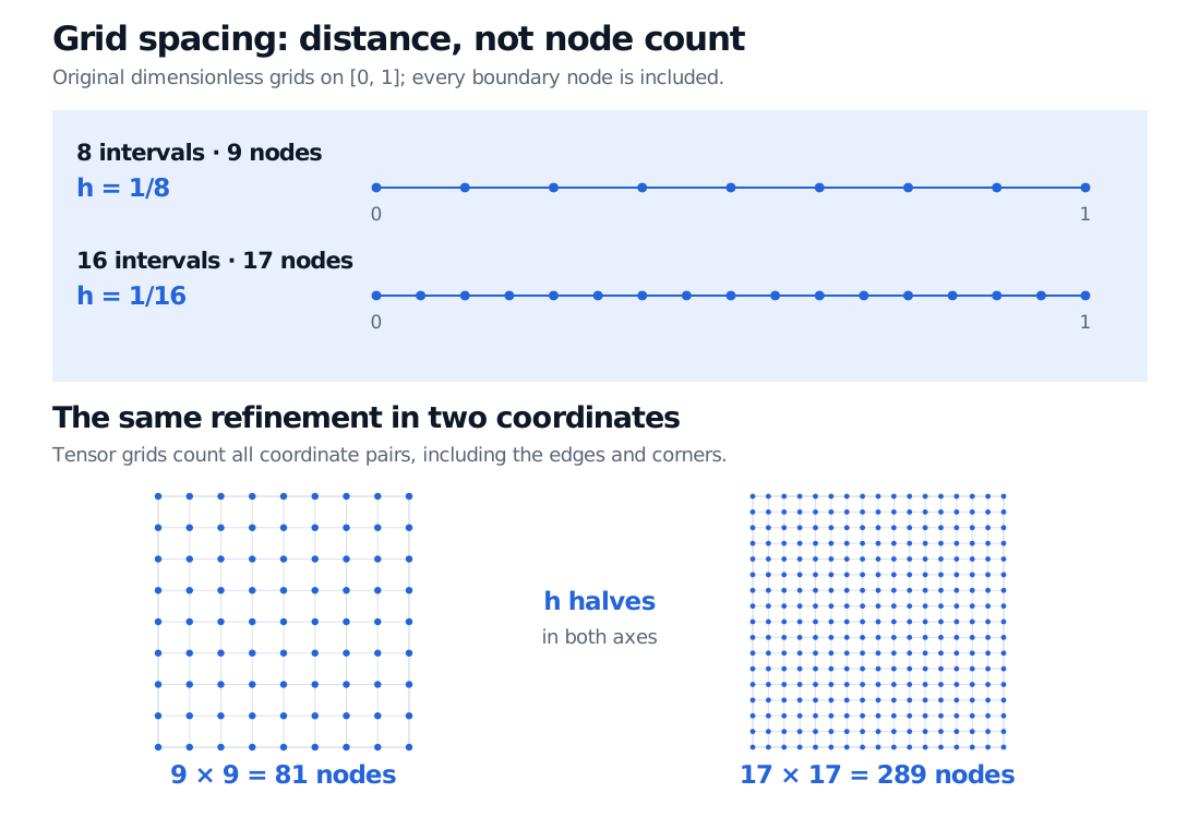
On [0,1], eight intervals give h=1/8 and nine nodes. Halving the spacing to 1/16 gives sixteen intervals and seventeen nodes. If the two boundary values are prescribed, the number of interior unknowns is seven and fifteen respectively.
Uniform grids on the unit interval have 8 intervals and 9 nodes at spacing 1/8, versus 16 intervals and 17 nodes at spacing 1/16. Endpoint-inclusive two-dimensional tensor grids have 9 by 9 equals 81 nodes and 17 by 17 equals 289 nodes.
Original dimensionless grids. Filled dots include all boundary nodes. Halving spacing in each coordinate changes both the one-dimensional resolution and the number of coordinate pairs.
For the square tensor grids shown, halving both coordinate spacings increases the node count from 92=81 to 172=289. This is not exactly four times as many nodes. On a fixed domain, a uniform tensor grid in d dimensions has node count proportional to h−d as h becomes small; halving every spacing therefore approaches a factor of 2d in node count. Actual runtime also depends on the solver, the number of time steps and how much of the grid is stored.
This is why fine grids become expensive for options with several state variables. A finer mesh buys resolution everywhere, even in regions that contribute little to the price of interest.
Smaller spacing can reduce one error
Take the synthetic dimensionless function f(x)=x3 at x=1, where the exact derivative is 3. A central difference uses two nodes, each a distance h from the target:
Dh=2hf(1+h)−f(1−h)=3+h2.
Spacing h
Sample nodes
Function values, left and right
Estimate Dh
Absolute error
0.2
0.8,1.2
0.512,1.728
3.04
0.04
0.1
0.9,1.1
0.729,1.331
3.01
0.01
These are exact decimal results in exact arithmetic. Halving h quarters this cubic's error. More generally, smooth central first differences have second order of accuracy. That is a statement about truncation error, not a promise that every grid refinement quarters the total pricing error.
In a real computation, closely spaced values can lose information through floating-point arithmetic, subtraction, or noise in the function evaluations. A payoff kink can also invalidate the smoothness assumption. The smallest available spacing need not give the best result.
Choose the coordinate and the domain as well
A uniform grid in log spot is not uniform in spot: equal increments in x=log(S/K) correspond to multiplicative changes in S=Kex, with fixed positive K. Report the coordinate alongside the spacing. For a nonuniform grid, use local gaps hi=xi+1−xi; a single mesh-size summary, often the largest gap, cannot describe where the resolution is concentrated. Difference weights must match those actual node locations.
Reducing spacing while keeping the outer boundaries fixed also leaves the domain truncation unchanged. If an option solver places an artificial boundary too close to the region of interest, refining inside that same domain does not remove the boundary error. Nor does spatial refinement alone ensure the time-stepping scheme is stable.
A useful pricing check compares results across several refinements while controlling the domain, boundary treatment and time discretisation. Compare the quantities needed for the decision: a price may look settled while a derivative estimated from nearby prices remains sensitive to resolution. The membership lesson Finite Difference Methods, available with a public preview, develops the spatial and time grids and their role in option-pricing schemes.
Sources
Rüdiger U. Seydel, Tools for Computational Finance, 6th edition, Springer, 2017, §1.3.3, §§4.2.1–4.2.2 and §4.7: grid dimensions, difference approximations, transformed coordinates and distinct numerical error sources.
Tobin A. Driscoll and Richard J. Braun, Fundamentals of Numerical Computation, Finite differences, §5.4: regularly spaced nodes and derivative stencils.
Driscoll and Braun, Convergence of finite differences, §5.5: spacing, order of accuracy and the competition between truncation and roundoff.