The Fisher z transformation maps a sample correlation to . It gives correlation inference a more convenient scale: under the usual bivariate-normal sampling model, the transformed coefficient has an approximately normal sampling distribution with a standard error that depends mainly on sample size. A quant comparing asset co-movement can use it to put uncertainty around an estimated correlation before treating that estimate as a portfolio input.
The transformation acts on a correlation coefficient, not on the individual returns. It neither makes the original data normal nor establishes a causal relationship.
Why change scale?
A correlation is bounded between −1 and 1. Its sampling distribution can be strongly skewed near those boundaries, making a symmetric error bar around a poor description. Fisher's transformation stretches the ends of the correlation scale:
The inverse is . Zero maps to zero, signs are preserved, and values approaching either boundary map towards positive or negative infinity. Consequently, an exactly perfect sample correlation cannot be fed into the finite- calculation. Check the data and sampling model rather than silently clipping the coefficient. Fisher's original discussion explicitly describes the resulting normality as an approximation. Fisher, §35
Suppose the observation pairs are independent and identically distributed from a nondegenerate bivariate normal distribution, with positive marginal variances and population correlation . The usual approximation is
Here is necessary for the displayed finite standard error; it does not guarantee accurate inference for every small sample. Finite-sample bias and departures from normality remain. Independence is across pairs; the two coordinates within each pair can be correlated. SciPy's maintained documentation states the bivariate-normal approximation and its standard error.
A correlation of 0.6 from 30 pairs
Take a hypothetical sample with and , under that model. No market data are being fitted here. To construct an approximate 95% confidence interval for :
- Transform: .
- Calculate .
- Form the interval on the transformed scale, using the standard-normal 97.5th percentile :
- Apply to both endpoints:
Calculations use unrounded intermediate values. The result is asymmetric around 0.6: the lower endpoint is about 0.294158 below it, while the upper is 0.189590 above it. This is the back-transformation doing its job, keeping the reported limits on the correlation scale. The interval construction follows the Stanford correlation-analysis summary.
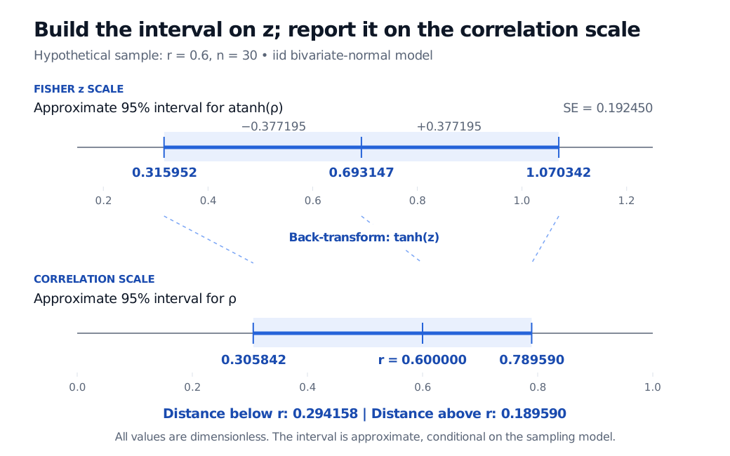
Original hypothetical example. The two axes use different linear scales; dashed guides connect corresponding endpoints and the estimate. The 95% interval relies on the stated sampling approximation.
“95%” describes the procedure's approximate coverage over repeated samples from the model. It is not a posterior probability that the fixed population correlation lies inside these realised limits. For that distinction and the connection to tests, see Confidence Intervals and Hypothesis Testing (public preview; full lesson requires membership).
Comparing correlations requires another independence check
For correlations estimated from independent samples, the usual approximate test of uses
Under the null and the corresponding sampling assumptions, is approximately standard normal. This is a standardised test statistic; a Fisher-transformed value by itself is not a standard-normal score. MedCalc's calculation details specify independent correlations.
Two assets' correlations with the same benchmark over the same dates are generally dependent estimates. Their comparison needs their covariance; the independent-sample denominator above is inappropriate. Overlapping return windows and serial dependence likewise invalidate blindly counting every row as an independent pair. A dependence-aware sampling model or suitably designed resampling procedure is needed; substituting an arbitrary “effective sample size” does not resolve the problem. A nonlinear transformation cannot create independence or remove outlier sensitivity.
Sources
- R. A. Fisher, Statistical Methods for Research Workers (1925), Chapter VI, §35, Transformed Correlations. Historical primary account of the transformation and its approximate sampling distribution.
- SciPy:
PearsonRResult.confidence_interval. Maintainer documentation of the Fisher interval and bivariate-normal standard-error approximation. - Afshine and Shervine Amidi, Stanford CME 106: Correlation analysis. Transformation and back-transformed confidence limits.
- MedCalc: Comparison of correlation coefficients. Fisher comparison for independent samples.