Build financial forecasts from operating inputs and separate a price change at fixed volume from an assumed customer response.
Driver-based financial forecasting
Driver-based financial forecasting projects financial results from explicit assumptions about what the business sells, uses or pays for. A distributor can forecast revenue from customer counts, units purchased per customer and realised selling prices. It can use the same unit forecast to estimate fulfilment costs. That gives the analyst something concrete to test when revenue grows but profit falls. Aswath Damodaran, Valuing Young, Start-up and Growth Companies, pp. 19–20, 28–29
Put the drivers on the same clock
A fictional distributor forecasts one month. It expects 1,000 distinct accounts to purchase during that month, at an average of three units per purchasing account. It expects a realised selling price of USD 20 per unit after discounts. For this example, all sales qualify for revenue recognition within the month.
1,000 accounts×3accountunits×20unitUSD=60,000 USD for the month.
Here, “active” means the account bought during the month, the same population used to measure the three-unit average. A month-end count of accounts with open contracts would give a different denominator. For a per-day usage driver, match the rate with account-days of exposure. For a quarter, build each month and add its revenue so that seasonal prices or usage rates apply in the right month.
Choose drivers that fit the business. A hotel can start from available room-nights, occupancy and price per occupied room-night. A manufacturer can forecast demand and cap shipments at the units it can supply. A top-down forecast starts with the addressable market and a market-share assumption. Compare the two on the same period and market definition. If the top-down result requires more rooms or production shifts than the business can supply, the forecast needs an explicit plan for adding capacity. Damodaran, pp. 19–22, 28–29
What changes when the price changes?
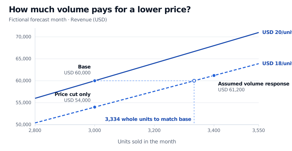
At USD 18 per unit and the same 3,000 units, monthly revenue falls to USD 54,000. That is a price sensitivity with volume held fixed. In a separate scenario, suppose the discount raises purchases to an average of 3.4 units per account and the account count stays at 1,000. With sufficient stock to deliver all 3,400 units, revenue reaches USD 61,200. The volume response is an input to that scenario. Estimating it would require evidence, such as a pricing test that separates the discount from seasonal demand. To find the volume needed to recover base revenue, divide USD 60,000 by USD 18 and round up to the next whole unit.
Revenue at 3,000 units falls from USD 60,000 at USD 20 per unit to USD 54,000 at USD 18 per unit. At USD 18, the forecast needs at least 3,334 whole units to match base revenue. An assumed increase to 3,400 units yields USD 61,200.
The guide line marks where USD 18 per unit recovers base revenue. The point at 3,400 units shows one assumed response.
If you measure each change against the base, the price cut costs USD 6,000 and the 400 extra units at the old price add USD 8,000. The extra units actually sell for USD 2 less each, so subtract another USD 800 to get the joint change of USD 1,200. In general, for base price P0, base quantity Q0 and changes ΔP and ΔQ, the exact bridge is
ΔR=Q0ΔP+P0ΔQ+ΔPΔQ.
A price-first bridge can instead value the extra 400 units at USD 18, which folds that interaction into the volume step. The total revenue change is identical.
Now assume a variable cost of USD 8 per unit and unchanged fixed costs. Revenue minus variable cost falls from USD 36,000 to USD 34,000 in the joint scenario. The extra sales cover the revenue lost to the discount, but their variable costs exceed the net revenue gain. In a three-statement model, carry the sales and cost assumptions into the operating forecast and model the timing of collections and payments separately.
Segment the forecast, then check it against actuals
Forecast channels or segments separately when prices, volumes or capacity constraints differ materially. Add the external revenue of each segment in a common currency. A shift toward a higher-priced product can raise the blended selling price even if every individual price stays fixed. If using a blended price, weight each price by its forecast units. Coca-Cola’s 2025 annual filing illustrates why this matters. Its historical revenue bridge reports volume separately from a combined price/mix measure that includes the effects of changes in products, channels and markets. The Coca-Cola Company, 2025 Form 10-K, Item 7, Net Operating Revenues
Keep the dated version of each forecast and the inputs available when it was made. Compare each version with the eventual actuals at the horizon the business uses, such as one month ahead. Check total revenue against a simple seasonal baseline, such as sales in the same month last year, then compare actual and forecast volume and price within each segment. Revenue can land on target when a volume miss and a price miss offset each other. Rebuilding the forecast with later-known sales or revised inputs introduces look-ahead bias. Hyndman and Athanasopoulos, Forecasting: Principles and Practice, §5.10