Understand a differential as a linear map of an input move, distinguish it from an actual valuation change, and keep units and stochastic notation consistent.
Differential
A differential is the linear map that turns an input increment into the first-order change of a differentiable function. If a valuation depends on a price S, its differential at the current price S0 is
dVS0(h)=V′(S0)h.
The derivativeV′(S0) is the sensitivity; the differential applies that sensitivity to a proposed move h. This is the calculation behind “sensitivity times price move” in a risk report. It estimates the effect of the scenario while holding other inputs fixed.
An equality that defines an approximation
The familiar notation dV=V′(S0)dS is an exact definition of the differential. The approximation enters when we use it for an actual finite change:
ΔV=V(S0+h)−V(S0)≈dVS0(h),dS=h.
At a fixed base point, doubling h doubles the differential. The actual valuation change need not double. Differentiability says that the omitted residual becomes negligible relative to the input move as that move tends to zero:
h→0lim∣h∣V(S0+h)−V(S0)−V′(S0)h=0.
A differential therefore need not be treated as a mysterious nonzero “infinitely small number.” Here, it is a linear rule evaluated on a chosen increment. Adding it to V(S0) gives the tangent-line estimate of the new level; the differential itself estimates the change.
A USD 1 price move: USD 2 or USD 2.01?
Consider the hypothetical valuation
V(S)=cS2,c=0.01USD−1.
Both S and V are measured in USD. The coefficient's inverse-currency units ensure that squaring a price still produces a dollar valuation. This is a teaching model, not a quoted instrument or a market-calibrated pricing formula.
At S0=USD 100, the value is USD 100 and the sensitivity is
V′(S0)=2cS0=2USD of inputUSD of value.
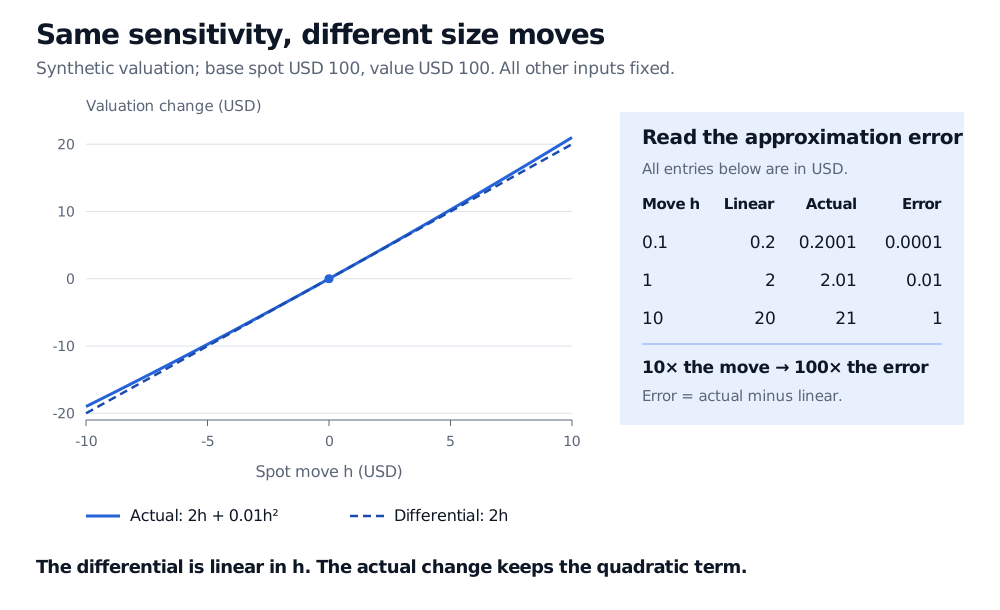
For a move to USD 101, set dS=h=USD 1. The differential gives dV=USD 2, so the tangent estimate of the new value is USD 102. Revaluing the model gives USD 102.01: the actual change is USD 2.01 and the linear estimate misses USD 0.01.
Expanding the square makes the distinction visible without any numerical approximation:
ΔV=2cS0h+ch2,dVS0(h)=2cS0h.
The omitted term ch2 is positive for either sign of a nonzero move. A fall of USD 1 therefore gives a linear change of minus USD 2, versus an actual change of minus USD 1.99. The estimate understates the value after both moves; “underestimate” does not mean it understates the magnitude of every loss.
At base spot USD 100, a USD 1 move gives differential USD 2 and actual change USD 2.01. A USD 10 move gives USD 20 and USD 21. Errors are USD 0.01 and USD 1.
Original synthetic valuation example. The chart holds the base sensitivity fixed; the table exposes the small residual that is hard to see near the tangent point. Error means actual change minus differential.
Here a tenfold move produces a hundredfold residual. More generally, a second-order Taylor expansion explains why curvature matters. This quadratic has no terms beyond second order, so its correction is exact. For a general valuation, adding a curvature term still leaves higher-order error. A price number alone does not tell you whether the linear estimate is accurate enough: the move, curvature and acceptable dollar error all matter.
Several inputs, one first-order change
For a differentiable scalar valuation of several inputs, the total derivative acts on the whole increment vector:
dVx(h)=i=1∑n∂xi∂V(x)hi=∇V(x)⊤h.
Each partial derivative holds the other inputs fixed; the differential adds their first-order effects. Every product must have the same output units. A sensitivity per unit of decimal volatility must multiply a decimal-volatility move, whereas a sensitivity per percentage point must multiply a percentage-point move. Mixing those conventions creates a factor-of-100 error.
The gradient collects these sensitivities. Joint finite moves can produce curvature and cross-effects that this linear sum omits. Merely having partial derivatives at a point does not by itself guarantee differentiability there.
When the symbol belongs to stochastic calculus
The d in dWt, for Brownian motion, belongs to stochastic-integral notation. It cannot be manipulated as an ordinary differentiable path increment. For a twice continuously differentiable function, Itô's lemma gives
df(Wt)=f′(Wt)dWt+21f′′(Wt)dt.
Dropping the second term by applying the ordinary chain rule loses an essential contribution. The ordinary differential remains useful for fixed-input scenario approximations; an equation for a function along a Brownian-driven process requires the stochastic rule.