Corrected cross-validation paired t-test: Definition & Examples

A corrected cross-validation paired t-test compares two learning procedures using paired validation-score differences while inflating the variance estimate to allow approximately for reuse of the same observations. The practical issue for a quant is false precision: running more overlapping train/test splits does not create more independent market histories.

This article uses the Nadeau–Bengio corrected resampled t-test convention. It adjusts uncertainty around an average score difference; it does not change either procedure’s measured scores.

Pair the experiment before correcting its uncertainty

Fit A and B on exactly the same training observations in each resample, and score both on the same held-out observations. For a higher-is-better metric such as accuracy, define $d_j=\text{score}_{A,j}-\text{score}_{B,j}$ . Positive differences favour A. For a loss metric, reverse the subtraction if positive is intended to mean improvement.

An ordinary paired t-test uses

s_d/\sqrt m

as the standard error of the mean of

m

differences. Repeated splits reuse observations, making unconditional score differences dependent even if split assignments were drawn independently. Treating the differences as independent can therefore understate uncertainty.

For the train/test split and refitting workflow, Cross-Validation and Information Criteria explains held-out model assessment and tuning (public preview; full lesson requires membership).

The correction, with its convention visible

Suppose every resample has $n_{\text{train}}$ training observations and $n_{\text{test}}$ test observations. Compute

\bar d=\frac{1}{m}\sum_{j=1}^{m}d_j, \qquad s_d^2=\frac{1}{m-1}\sum_{j=1}^{m}(d_j-\bar d)^2, \qquad r=\frac{n_{\text{test}}}{n_{\text{train}}}.

The corrected statistic for a zero expected score difference is

\widehat{\text{SE}}_{\text{corr}} =\sqrt{\left(\frac{1}{m}+r\right)s_d^2}, \qquad T_{\text{corr}}=\frac{\bar d}{\widehat{\text{SE}}_{\text{corr}}}.

Here

m

counts resamples, not observations in the original dataset. The calculation needs

m\ge2

and positive

s_d^2

. Its target is the expected score difference between procedures trained on

n_{\text{train}}

observations, which need not equal their difference after training on the full dataset. The reference convention is Student’s t-distribution with

m-1

degrees of freedom. A two-sided p-value uses both tails beyond

\lvert T_{\text{corr}}\rvert

Nadeau and Bengio motivate the added term by approximating the correlation between split-level estimates as

\rho_0=n_{\text{test}}/(n_{\text{train}}+n_{\text{test}})

, giving

\rho_0/(1-\rho_0)=r

. This is a surrogate correlation, not an estimate measured from the ten scores. Their 2003 paper, §§3.1 and 4, method 6, makes the approximation explicit: actual correlation above the surrogate can still make inference too liberal; below it, inference can be conservative. The t reference is consequently approximate outside the paper’s ideal Gaussian correlation model.

Ten resamples, one apparent advantage

Take these fictional accuracy differences, expressed as fractions rather than percentages:

(0.01,\ 0.02,\ 0,\ 0.03,\ 0.02,\ 0.01,\ {-0.01},\ 0.02,\ 0.03,\ 0.01).

Each resample uses 80% of the observations for training and 20% for testing, so $r=0.25$ . These are stipulated score summaries, not empirical evidence for a financial strategy.

The mean is

\bar d=0.014

, or 1.4 percentage points, and the sample variance is

s_d^2=0.00016

. Thus

\widehat{\text{SE}}_{\text{corr}} =\sqrt{(0.1+0.25)(0.00016)} \approx0.0074833, \qquad T_{\text{corr}}\approx1.87083.

With nine reference degrees of freedom, the approximate two-sided p-value is 0.09417. An analysis using a prespecified 5% threshold would not reject the zero-mean null. This does not establish equality of the procedures.

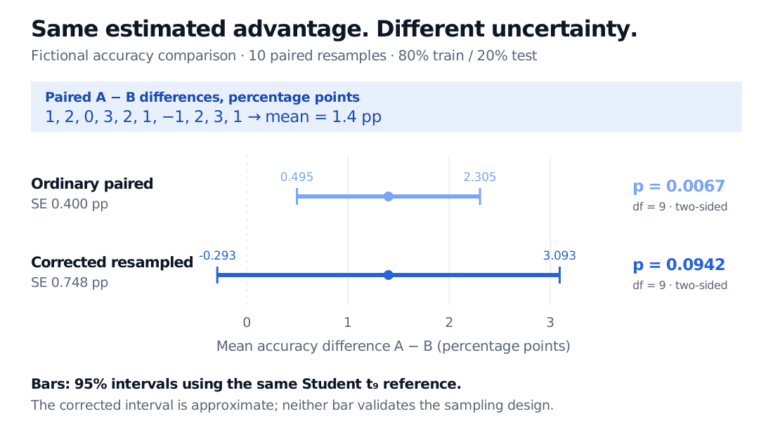
The ordinary paired calculation instead gives $\text{SE}=0.004$ , $T=3.5$ and $p\approx0.00672$ . The correction multiplies the variance estimate by $3.5$ and the standard error by $\sqrt{3.5}\approx1.871$ . The same measured advantage now carries substantially more uncertainty.

Fictional mean accuracy advantage is 1.4 percentage points. The ordinary 95% interval is 0.495 to 2.305 pp, with SE 0.400 pp and p 0.0067. The corrected interval is minus 0.293 to 3.093 pp, with SE 0.748 pp and approximate p 0.0942; both use nine reference degrees of freedom.

Original fictional comparison. Both bars use the same Student t critical value; the corrected 95% interval crosses zero. Its coverage remains an approximation under the stated resampling convention.

Holding the observed $s_d^2$ and split ratio fixed, the corrected formula’s standard error approaches $\sqrt{r s_d^2}$ as $m$ increases, rather than zero. This algebra explains why repeated repartitioning cannot substitute for collecting fresh data; it does not assert that the observed variance stays fixed in an actual experiment.

Identify the design before borrowing the formula

In repeated k-fold cross-validation, each full repetition supplies

k

fold scores. With

R

repetitions, a fold-level correction uses

m=Rk

and, for equal folds,

r=1/(k-1)

. Bouckaert and Frank (2004), §3.3, describe a corrected repeated-k-fold statistic using this structure, with the fold-level

Rk-1

reference convention. A full repetition is not one fold-level observation; analysing repetition averages would require a separately justified variance model and degrees of freedom. State the variance estimator, counting unit and reference degrees of freedom when reporting a variant; a shared test name does not make every resampling design equivalent. The worked example above uses ten repeated holdouts and the

m-1=9

corrected-resampling reference.

For financial prediction, the underlying independent-data framework needs particular scrutiny. Autocorrelation, overlapping labels and changing market regimes are additional dependence problems. Purged cross-validation addresses training/test label overlap; it does not automatically validate this t reference. Preprocessing and tuning must respect training boundaries, because increasing a denominator cannot remove information leakage.

Finally, comparing the winning pair after searching many models introduces multiple testing in strategy research. This correction does not account for that search. Report the paired effect, metric, split design, tuning process and comparison family alongside the p-value. Accuracy evidence alone also says nothing about turnover, transaction costs or tradable profitability.

Sources

Nadeau, C., and Bengio, Y. (2003), Inference for the Generalization Error, Machine Learning 52, 239–281: §1 defines the resampling experiment; §3.1 derives the variance correction; §4, method 6, states the corrected resampled t reference and its limitations.
Nadeau and Bengio, Inference for the Generalization Error, NeurIPS 1999 conference version: earlier treatment in §3; distinct from the expanded 2003 journal article.
Bouckaert, R. R., and Frank, E. (2004), Evaluating the Replicability of Significance Tests for Comparing Learning Algorithms: §§3.2–3.3 distinguish random subsampling from repeated k-fold scores.

Pair the experiment before correcting its uncertainty

The correction, with its convention visible

Ten resamples, one apparent advantage

Identify the design before borrowing the formula

Sources

Related terms

P-value

Paired t-test

Standard error

Student's t-distribution