Confidence level is the coverage target of an interval procedure. Compare 90%, 95% and 99% mean-slippage intervals and learn what their percentages do—and do not—say.
Confidence level
A confidence level is the target repeated-sampling coverage of a procedure for estimating an unknown parameter. A 95% confidence interval procedure is designed to include the true parameter in at least 95% of repeated applications under its stated assumptions. The percentage describes the procedure, rather than a probability assigned to a fixed parameter after seeing one interval.
For an execution desk estimating average slippage, this matters immediately: raising confidence can widen the uncertainty range enough to change whether the evidence supports a cost budget.
What carries the 95%?
Let θ be a fixed population parameter and let [L(X),U(X)] be an interval calculated from random sample X. A level-(1−α) procedure satisfies
Pθ(L(X)≤θ≤U(X))≥1−α
for every parameter value in its stated model. Here α is the allowed noncoverage probability. Exact 95% coverage means equality at 0.95; conservative procedures can cover more often. An approximate 95% interval instead relies on an approximation whose accuracy needs justification. The printed nominal level is not evidence that actual coverage survives a wrong sampling model.
Before sampling, the endpoints vary with the data. After sampling, they become numbers, while the unknown parameter remains fixed. We usually cannot tell whether this particular interval contains it. Frequentist coverage alone does not supply a 95% posterior probability for that event; a credible interval requires a Bayesian model. Nor does 95% mean that this interval contains 95% of observed trades or 95% of future slippage outcomes. Those are questions about observations, rather than uncertainty about their population average.
One cost study, three confidence levels
Consider a hypothetical study of 36 same-horizon executions. Slippage is measured against the same benchmark, with positive basis points representing a cost. Assume independent, identically distributed normal observations, an unknown unchanged mean μ, and a known population standard deviation of 1.5 bp. Known variability is a simplifying model assumption here, not something established by these 36 trades.
The observed sample mean is 5.2 bp. Its standard error is σ/n=1.5/6=0.25 bp. Since
σ/nXˉ−μ∼N(0,1),
a two-sided, equal-tailed interval is
xˉ±z1−α/2nσ,
where zp is the standard-normal p-quantile. For 95% confidence, α=0.05 leaves 0.025 in each tail, giving the critical valuez0.975≈1.959964. Thus the interval is 5.2±0.489991 bp, or approximately [4.710, 5.690] bp.
Confidence level
Critical value
Margin of error (bp)
Mean-slippage interval (bp)
90%
1.644854
0.411213
[4.789, 5.611]
95%
1.959964
0.489991
[4.710, 5.690]
99%
2.575829
0.643957
[4.556, 5.844]
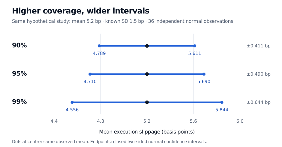
Three nested confidence intervals for the same observed mean of 5.2 basis points: 90% from 4.789 to 5.611, 95% from 4.710 to 5.690, and 99% from 4.556 to 5.844. All use 36 iid normal executions and known population standard deviation 1.5 basis points.
Original hypothetical execution study. Holding the data, model and equal-tailed construction fixed, higher coverage requires wider intervals. The black dots all mark the same observed mean.
Suppose a desk requires the two-sided interval's upper endpoint to lie below a predeclared ceiling of 5.7 bp. The 95% interval passes that rule, while the 99% interval does not. Neither result guarantees that an individual trade costs less than 5.7 bp. If the desk instead needs a one-sided upper confidence bound, it should specify that design beforehand; its cutoff differs from the two-sided one used here.
The width comparison holds within this fixed construction. A confidence level alone does not rank widths across different datasets, sample sizes, models or interval methods. More independent observations can offset the wider critical value. Replacing the known population SD with an estimated sample SD also changes the exact normal-family calculation to a Student t interval.
Choose the procedure before the result
A 95% label belongs to the whole sampling and analysis rule. Correlated executions, changing liquidity conditions or heavy-tailed slippage can undermine the normal iid guarantee. Choosing the confidence level after inspecting which interval clears the budget changes the reporting rule; repeatedly sampling until an endpoint looks attractive also needs a sequentially valid design. The nominal percentage does not automatically protect either practice.
For the normal-family derivation and its connection to hypothesis tests, continue with Confidence Intervals and Hypothesis Testing. It has a public preview; full access requires membership.
Sources
Larry Wasserman, All of Statistics: A Concise Course in Statistical Inference, Springer, §6.3.2, pp. 92–93: confidence sets, coverage and the distinction between a random interval and a fixed parameter.