A density-forecast diagnostic using normal-transformed forecast percentiles. Understand the joint mean, variance and AR(1) test, likelihood conventions and its limits.
Berkowitz test
The Berkowitz test is a likelihood-ratio diagnostic for density forecasts: it converts each realised outcome's forecast percentile into a standard normal score, then tests restrictions on that score's mean, variance and first-order serial dependence. A risk model can predict the frequency of value-at-risk breaches reasonably well while misrepresenting the rest of the loss distribution. Using the forecast distribution gives the validator more information than a breach indicator alone.
Put different forecasts on the same scale
Suppose Ft is the one-step-ahead forecast cumulative distribution function for outcome Yt, issued using information available before Yt is observed. Compute
ut=Ft(Yt),zt=Φ−1(ut),
where Φ is the standard normal CDF. The first step is the probability integral transform, or PIT. If the continuous conditional forecast distribution is correct given the preceding information, the PIT sequence is independent uniform on (0,1); the normal scores are consequently independent N(0,1). A correct unconditional distribution alone does not establish this independence. Diebold, Gunther and Tay's original density-evaluation paper, §3, gives the conditional argument.
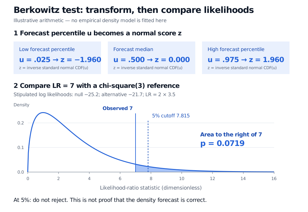
For example, a realisation at the forecast median has ut=0.5 and zt=0. At the 97.5th forecast percentile, zt≈1.959964. These are forecast-relative scores: a large dollar loss need not have an extreme score if the forecast already assigned substantial probability to such losses. The observed P&L itself need not be normally distributed.
Three restrictions, one comparison
Use the Gaussian first-order autoregressive model
zt=m+ρ(zt−1−m)+εt,εt∼iidN(0,v),v>0,∣ρ∣<1.
Here m is the stationary mean and v is the innovation variance. The stationary variance is v/(1−ρ2), rather than v in general. The joint null is
H0:m=0,v=1,ρ=0.
This article uses the exact stationary Gaussian likelihood, including the first score's density. If φa(x) denotes the zero-mean normal density with variance a, its log likelihood is
Maximise this likelihood over (m,v,ρ) for the alternative and evaluate it at (0,1,0) for the null. The likelihood-ratio test statistic is
LR3=2[ℓ(m^,v^,ρ^)−ℓ(0,1,0)].
Under the regular null, its large-sample reference distribution is χ32: three restrictions are imposed. This is the joint test developed in Berkowitz's original working paper, §3a, subsequently published in 2001.
A conditional-likelihood variant drops the initial-density term and conditions on z1. It must use that same convention, observation window and normalising constants for both fits; mixing an exact null likelihood with a conditional alternative likelihood does not produce the stated statistic.
Read a result without overclaiming
For an arithmetic illustration, stipulate comparable maximised log likelihoods of −25.2 under the null and −21.7 under the alternative for the same score series and likelihood convention. These are illustrative inputs, not estimates from market data. Then
LR3=2[−21.7−(−25.2)]=7,p=P(χ32≥7)≈0.07190.
At a prechosen 5% level, do not reject; the 5% reference cutoff is approximately 7.815. This p-value is not the probability that the forecast model is correct.
Illustrative normal-score mapping: forecast percentiles 0.025, 0.5 and 0.975 become minus 1.960, zero and 1.960. Stipulated log likelihoods minus 25.2 and minus 21.7 give LR3 equal to 7; the chi-square distribution with three degrees of freedom has right-tail area 0.0719 beyond 7, below the 5% cutoff of 7.815.
Original arithmetic illustration. The shaded region is the asymptotic p-value beyond LR3 = 7; no empirical density forecast has been fitted.
A separate AR(1) dependence comparison allows the mean and innovation variance to be fitted under both hypotheses, restricts only ρ=0 under its null, and uses a χ12 reference under regularity. It answers a different question from LR3. Re-estimate the nuisance parameters under the restriction; simply setting an unrestricted estimate of ρ to zero is insufficient.
The joint test is sensitive to the departures represented by its Gaussian AR(1) alternative. It does not establish every aspect of normality or independence. Nonlinear dependence, higher-lag structure and incorrect tail shape can remain even when the mean, variance and first-order correlation look acceptable. Inspect PIT plots, dependence in transformed powers and tail-specific diagnostics alongside it.
What can invalidate the comparison?
Atoms: for discrete or mixed forecasts, Ft(Yt) is generally not uniform. A declared randomised PIT uses ut=Ft(Yt−)+Vt[Ft(Yt)−Ft(Yt−)], with independent Vt∼U(0,1). Record the randomisation and its seed; Dunn and Smyth (1996), §3, give this construction.
Endpoints:Φ−1(0) and Φ−1(1) are infinite. Silently clipping PITs makes scores finite by changing the data and can conceal tail failures. Investigate support and numerical precision, and disclose any approximation.
Evaluation design: fitting a model on its evaluation outcomes, parameter-estimation uncertainty, or overlapping multi-period outcomes can alter the reference law. Preserve forecast timestamps and use inference suited to that design; the one-step independent-score argument does not automatically cover overlapping horizons.
For the restricted-versus-unrestricted fitting principle, see The Generalized Likelihood Ratio Test (public preview; full lesson requires membership).