How Bayesian neural networks carry weight uncertainty into predictions, distinguish function spread from observation noise, and depend on approximate inference and calibration.
Bayesian neural network
A Bayesian neural network (BNN) is a neural network whose uncertain parameters are assigned a prior and updated using data to obtain a posterior distribution. Predictions average over that parameter uncertainty. For a quant forecasting returns or default events, this can distinguish disagreement about the fitted prediction rule from variability in the outcome—even after fixing the rule.
The Bayesian treatment concerns the model's unknown quantities, commonly its weights and biases. It does not require a different neural architecture. A Bayesian network, despite the similar name, is a graphical model of conditional dependencies; it is a different concept.
A distribution over weights becomes a distribution over predictions
Write the network's parameters as w, its output function as fw(x), and the training data as D. A priorp(w) specifies parameter beliefs before those data. A likelihoodp(D∣w) describes the observed targets conditional on their inputs and parameters. Bayes' rule gives the posterior:
p(w∣D)∝p(D∣w)p(w).
The likelihood also determines what the network output means: it may be a conditional mean for regression or parameters of a class-probability distribution. The posterior predictive distribution for a new observation averages the entire conditional observation distribution:
p(y∗∣x∗,D)=∫p(y∗∣x∗,w)p(w∣D)dw.
These are the posterior and prediction constructions developed in Jospin and coauthors' BNN tutorial, Section II. Drawing a parameter vector and evaluating its network produces one possible function. Drawing an observation from that function's likelihood adds outcome variability. Those are distinct operations.
Two possible weights, two kinds of spread
Consider the deliberately minimal scalar function fw(x)=wx. It isolates the uncertainty calculation without hidden layers. Stipulate the entire posterior: weight w=1 has probability 1/2, and weight w=3 has probability 1/2. No data have been fitted to obtain these probabilities. All quantities are dimensionless.
At x∗=2, the two possible function values are 2 and 6. Their posterior mean and variance are
The halves are probability weights for a complete two-point distribution. This is a population variance, not an unbiased sample-variance estimate from two Monte Carlo draws; an n−1 denominator would answer a different question.
Now specify independent conditional observation noise with variance 1:
y∗∣x∗=2,w∼N(2w,1).
The second normal parameter denotes variance. The future observation therefore has the mixture distribution
y∗∣x∗=2,D∼21N(2,1)+21N(6,1).
Its mean remains 4, but its variance is 5. The law of total variance explains the extra spread:
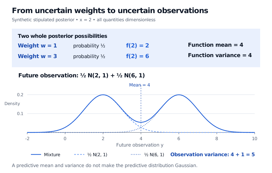
A stipulated posterior assigns weights 1 and 3 probability one half each. At input 2 the function values are 2 and 6, with mean 4 and variance 4. The future-observation density is an equally weighted mixture of normals with means 2 and 6 and variance 1 each; its mean is 4 and total variance is 5.
Original synthetic example. Dashed and dotted curves show the probability-weighted component densities; the solid curve is their sum. Observation variance equals function variance 4 plus conditional noise variance 1.
The mixture is not N(4,5). Matching its mean and variance would discard its two-peaked shape. In a nonlinear network, averaging parameters and then evaluating the network also need not equal averaging the networks' predictions.
In this specified regression model, variation in the conditional mean across posterior parameters represents epistemic uncertainty about the function. Expected conditional observation variance represents aleatoric uncertainty remaining at fixed parameters and inputs. This split is conditional on the chosen model and information: a richer input set or a different noise specification can change what gets classified as residual noise. It does not measure every source of uncertainty about a financial forecast.
How a practical posterior is obtained
Exact posterior computation is usually difficult for a large network. Variational inference replaces the posterior with a tractable distribution qθ(w). Bayes by Backprop, introduced by Blundell and coauthors, learns such a distribution using stochastic gradients. Its objective is
KL(qθ(w)∥p(w))−Eqθ[logp(D∣w)].
This balances an expected likelihood term against divergence from the prior. A diagonal Gaussian approximation, for example, cannot capture posterior dependence between weights. Drawing more predictions from the same approximation reduces simulation error; it does not remove that restriction or repair model misspecification. Markov chain Monte Carlo offers another inference route, with its own computational and convergence checks.
A single maximum a posteriori weight vector retains a posterior mode rather than the distribution. Likewise, several independently trained networks are not automatically posterior samples merely because their outputs are averaged.
A forecast distribution still needs evidence
A prior, likelihood and inference algorithm together determine the reported uncertainty. A narrow approximate posterior can reflect restrictive assumptions or missed posterior regions. It need not establish that the market outcome is predictable.
Evaluate forecasts on later eligible data, using only information available at each fit and decision time. Examine predictive density scores and interval coverage alongside interval width; wide intervals can achieve coverage while offering little useful resolution. Check performance across relevant market conditions. These are evaluation choices for the proposed financial application, not conclusions established by the synthetic example.
Calibration on one distribution does not guarantee calibration after a shift.Ovadia and coauthors compare uncertainty methods on classification benchmarks under dataset shift, including variational BNN methods. Their evidence motivates testing uncertainty under changed conditions; it does not establish reliability for financial returns. A BNN has no general guarantee that unfamiliar inputs will trigger sufficiently high uncertainty.
For the underlying updating mechanics, Bayesian Reasoning works through explicit prior–likelihood–posterior calculations and prior strength. Its preview is public; the full lesson requires membership.
Sources
Blundell, Cornebise, Kavukcuoglu and Wierstra (2015), Weight Uncertainty in Neural Networks, Sections 2–3.2: point estimates, posterior prediction, the variational objective and Bayes by Backprop.
Jospin, Laga, Boussaid, Buntine and Bennamoun (2022), Hands-on Bayesian Neural Networks—A Tutorial for Deep Learning Users, Section II: Bayesian parameter modelling and posterior prediction. The two-point example and variance calculation here are original stipulated constructions.