Compare traded-factor pricing models through excluded-factor alphas and Sharpe spanning. Separate the exact population identity from Bayesian model probabilities.
Barillas-Shanken model comparison
Barillas-Shanken model comparison evaluates competing asset-pricing models by asking how well their traded factors price the factors excluded from each model. For a quant choosing between factor sets, this shifts attention from a leaderboard of test-portfolio errors to the investment opportunities that one factor set leaves unexplained.
Two related contributions need separating. Which Alpha? (2017) develops the excluded-factor and Sharpe-spanning logic. Comparing Asset Pricing Models (2018) builds a Bayesian procedure for assigning model probabilities. A Sharpe improvement alone is neither a significance test nor a posterior probability.
First hedge away what the existing factors explain
Let F be a vector of traded excess-return factors and G another traded excess return, all measured over the same period. In the population linear regression
G=α+βTF+ε,E[ε]=0,Cov(F,ε)=0,
alpha is the mean return left after hedging the exposure to F. The traded hedge G−βTF has mean α and variance σε2; the regression disturbance itself has zero mean.
For an excess-return vector X with mean μX and positive-definite covariance matrix VX, the maximum squared Sharpe ratio over unrestricted linear portfolios is
S2(X)=μXTVX−1μX.
The spanning identity is
S2(F,G)−S2(F)=σε2α2.
This uses finite second moments, nonsingular covariances and frictionless positions, including shorting and cash financing. It needs no normal-distribution assumption. With several excluded factors, replace the scalar ratio by αTVε−1α, which accounts for covariance between their residuals. These are mean-variance statements: zero alpha means no additional maximum Sharpe, even if the factor has substantial residual risk. It does not mean its payoff is exactly replicated.
The Risk-Adjusted Performance Measures lesson develops the related appraisal ratio, alpha per unit of residual risk. Its preview is public; the full lesson requires membership.
A second factor with a smaller standalone mean can still help
Consider fictional monthly population moments for two traded excess-return factors. Returns are decimals; every entry uses the same monthly horizon:
μ=(0.0050.004),V=(0.00040.000120.000120.0009).
The monthly means are 0.5% and 0.4%. Factor F1 alone gives
S2(F1)=0.00040.0052=0.0625.
Regress F2 on a constant and F1. The population slope, intercept and residual variance are
Directly calculating μTV−1μ gives the same joint value. The gain is in squared Sharpe units, not percentage points of return. No annualisation is being applied.
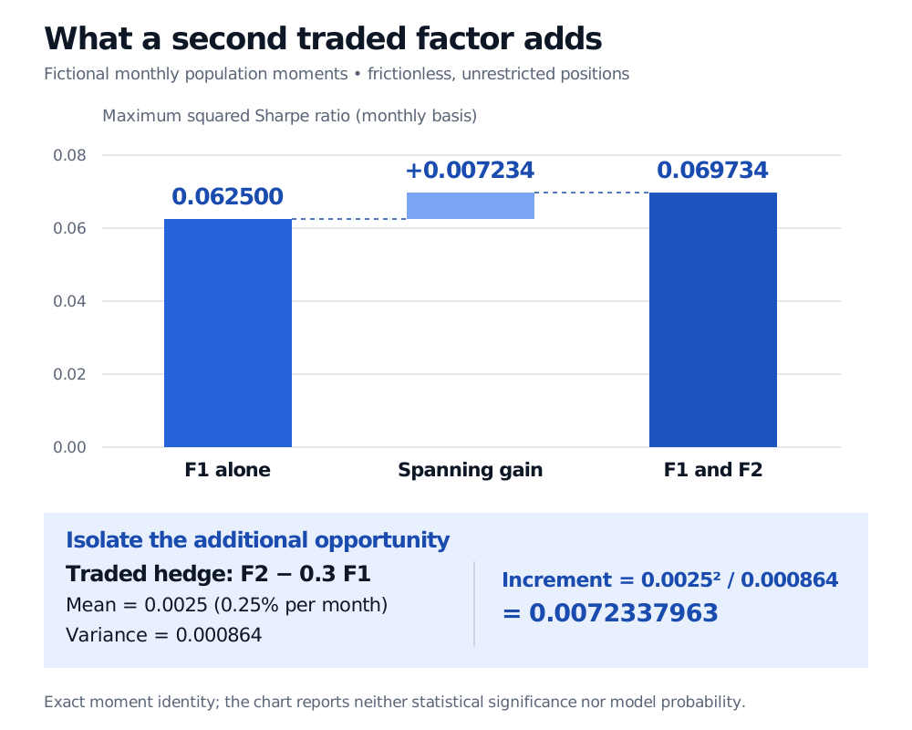
Fictional monthly population maximum squared Sharpe is 0.062500 for F1 alone. The traded hedge F2 minus 0.3 F1 has mean 0.0025 and variance 0.000864, contributing 0.0072337963. Together F1 and F2 achieve 0.0697337963. The gain is an exact moment identity, not a posterior probability.
Original fictional monthly population calculation with unrestricted, frictionless positions. The light-blue bridge is alpha squared divided by residual variance; it measures the added investment opportunity after hedging F1 exposure.
These supplied moments establish a population opportunity. They provide no sample size, sampling uncertainty or probability that a model is correct.
What “test assets are irrelevant” actually requires
In Which Alpha?, the comparison includes the union of both models’ traded factors, alongside common test assets. Under the Sharpe-improvement criterion, the gain from adding test assets to that union is common to both models and cancels. For its likelihood result, joint returns are elliptically distributed with finite second moments, the relevant conditional densities are linear regressions, and parameters not restricted by the models are held fixed. The common test-asset likelihood then cancels; arbitrary error scores need not share that property.
Test assets still assess absolute pricing adequacy. A relative winner can leave large pricing errors. Nontraded macroeconomic quantities also require care: their mimicking portfolios depend on available asset returns, so the test assets used to identify those portfolios can affect the comparison. Consumption growth cannot simply be inserted into a traded-return Sharpe calculation.
From spanning to Bayesian comparison
Comparing Asset Pricing Models integrates likelihoods over parameter priors, then combines those marginal likelihoods with model priors:
P(Mj∣D)=∑kp(D∣Mk)P(Mk)p(D∣Mj)P(Mj).
Every model must account for the same dataD, including excluded factors. The paper specifies proper priors for alpha under the alternative, with prior scale linked to plausible Sharpe improvements. Its tractable Bayesian results assume conditionally normal residuals independent over time, with constant residual covariance and independent prior blocks for the component regressions. Prior choices matter; the posterior probabilities are conditional on the candidate universe and statistical specification.
In a nested sample comparison, expanding the unrestricted portfolio set cannot lower its maximised sample squared Sharpe: retaining the old portfolio is always feasible. An apparent improvement can therefore reflect estimation noise. The population identity above supplies no automatic sample winner, no Bayes factor, and no evidence about trading costs or performance on future observations.
Sources
Francisco Barillas and Jay Shanken, Which Alpha?, Review of Financial Studies 30(4), 1316–1338 (2017), especially §1 and equation (4), §2 Proposition 2, and §4.1. The NBER record links the earlier working-paper version.