Wavelet analysis: Definition & Examples

Wavelet analysis decomposes a signal into components associated with different scales and positions in time. For a quant, it can distinguish a brief burst of variation from a slower change that spans many observations. The decomposition describes the supplied data; it does not by itself identify an economic cause or produce a tradable forecast.

A global Fourier transform uses oscillations extending across the record. Wavelets use shifted, stretched versions of a localised function: a short version responds to fine changes, while a stretched version spans broader changes. A periodogram summarises frequency content over its chosen window; wavelet analysis makes the position within that window part of the description. Localisation comes with a trade-off: sharpening time resolution blurs frequency resolution, and vice versa. Torrence and Compo, §3 explain this balance.

A complete four-observation transform

The Haar wavelet makes the mechanism visible with sums and differences. Take the synthetic signal

x=(1,1,3,3)

, sampled at equal intervals in arbitrary units. Fix nonoverlapping adjacent pairs starting at the first observation. For every pair

(u,v)

, calculate

a=\frac{u+v}{\sqrt{2}},\qquad d=\frac{u-v}{\sqrt{2}}.

Here

a

is a low-frequency or approximation coefficient and

d

is a detail coefficient. The divisor

\sqrt{2}

makes this an orthonormal transformation: the two new directions are perpendicular and have unit length. These are normalised sums, not ordinary pair averages. The sign convention is left minus right; reversing that convention reverses detail signs without changing the information.

At the first level,

a_1=(\sqrt{2},3\sqrt{2}),\qquad d_1=(0,0).

Both within-pair differences vanish. Apply the same operation to the two entries of $a_1$ :

a_2=\frac{\sqrt{2}+3\sqrt{2}}{\sqrt{2}}=4, \qquad d_2=\frac{\sqrt{2}-3\sqrt{2}}{\sqrt{2}}=-2.

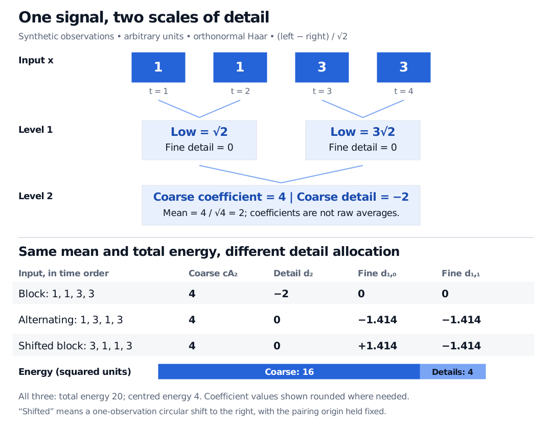
The complete representation contains four numbers: one coarse coefficient

a_2=4

, one coarse detail

d_2=-2

, and two fine details equal to zero. It retains the four input degrees of freedom; downsampling has not discarded information because both branches were kept. This is the multilevel approximation/detail structure described in the official DWT documentation.

Haar transform of the synthetic signal 1, 1, 3, 3 gives coarse coefficient 4, coarse detail minus 2 and fine details zero; alternating and circularly shifted signals retain mean 2 and energy 20 but change detail coefficients.

Haar analysis preserves all four observations while separating broad and fine differences. The same mean and energy can coexist with different allocations across scales.

Reconstructing the observations

The inverse of each pair operation is

u=\frac{a+d}{\sqrt{2}},\qquad v=\frac{a-d}{\sqrt{2}}.

First reconstruct the low coefficients as $(4-2)/\sqrt{2}=\sqrt{2}$ and $(4+2)/\sqrt{2}=3\sqrt{2}$ . Combining each with its zero fine detail then returns $(1,1)$ and $(3,3)$ . No smoothing has occurred yet. Dropping or shrinking details would change the reconstructed signal and requires a separate choice about what counts as noise.

The normalisation also preserves squared Euclidean energy:

1^2+1^2+3^2+3^2 =20 =4^2+(-2)^2+0^2+0^2.

Energy here means sum of squares in squared signal units, not financial risk capital or automatically a variance. The arithmetic mean is $2$ , not $4$ : for this four-point complete Haar decomposition,

\bar{x}=a_2/\sqrt{4}

. Removing the mean leaves centred energy

4

, exactly the sum of squared detail coefficients. A variance would additionally require its stated divisor.

Compare $y=(1,3,1,3)$ . Its coarse coefficient is again $4$ , but $d_2=0$ and $d_1=(-\sqrt{2},-\sqrt{2})$ . Its total energy is also $20$ . The first series changes between the two halves; the second changes inside both pairs. Equal mean and energy do not imply equal temporal structure.

Discrete and continuous analyses answer different questions

Approach	What is retained	Useful interpretation
Discrete wavelet transform (DWT)	A hierarchy of approximation and detail coefficients; the usual filter bank downsamples each branch	A compact multiscale representation, with reconstruction when the required coefficients and conventions are retained
Continuous wavelet transform (CWT), evaluated on a grid	Many overlapping shifts and scales	A redundant time–scale map; squared coefficient magnitudes are often displayed as a scalogram

For the CWT, a common continuous-time convention is

W_x(a,b)=\frac{1}{\sqrt{a}}\int_{-\infty}^{\infty} x(t)\,\overline{\psi\!\left(\frac{t-b}{a}\right)}\,dt, \qquad a>0.

Here

a

stretches the mother wavelet

\psi

b

locates it in time, and the bar denotes complex conjugation. Larger scales span longer intervals. A scale is not a universal frequency label: converting it to cycles per day needs the chosen wavelet and sampling interval. Software may normalise coefficients in sample units rather than physical-time units, so colour magnitudes are not interchangeable across conventions. The official CWT documentation states both its scale-to-frequency mapping and coefficient convention. The finite orthonormal energy identity above must not be copied unchanged to a redundant scalogram. Adding more scales does not defeat the sampling limit; excessively small scales can introduce discretisation or aliasing artifacts.

Choices that can change the conclusion

Pairing origin and downsampling. Circularly shifting the block signal one observation to the right gives

(3,1,1,3)

. With the same pairing origin, its coarse detail becomes zero and its fine details become

(\sqrt{2},-\sqrt{2})

. An ordinary decimated DWT is sensitive to shifts. Undecimated approaches retain more coefficients to address this sensitivity; the stationary wavelet transform documentation describes the modification. Its name does not establish stationarity of the input process.

Record boundaries. Our four-point Haar example needs no extension. Longer filters or other record lengths can require values beyond the observed endpoints. Zero padding, reflection and periodic extension encode different assumptions and can create different edge details. Reconstruction must use compatible conventions. The official extension-mode documentation illustrates these artifacts. In CWT work, the cone of influence marks a convention-dependent region where edge effects matter; it is not a statistical confidence region.

Information available at the decision time. Even a local coefficient may use future data relative to its plotted timestamp. In our example, the first fine detail requires both

x_1

and

x_2

: it cannot be known after observing

x_1

alone. A centred filter or full-record reconstruction can likewise introduce look-ahead bias. For forecasting, recompute features using only data available at each origin, timestamp them after their required inputs arrive, and select wavelets, levels and denoising rules within the training procedure.

The object being analysed. Prices, returns and squared returns encode different questions. A large coefficient in a price level is not automatically a volatility spike; a broad component is not automatically a persistent economic cycle. Specify sampling, adjustments, missing-data handling and the input transformation before interpreting the scales. Searching many time–scale cells or wavelet choices also creates a multiple-testing problem: a striking patch alone is insufficient evidence of a repeatable pattern.

Sources

Torrence and Compo (1998), A Practical Guide to Wavelet Analysis, §§3a, 3e, 3g–h: localisation, resolution, edge effects and scale versus frequency.
PyWavelets: Discrete Wavelet Transform, single-level and multilevel approximation/detail structure.
PyWavelets: Continuous Wavelet Transform, transform convention, normalisation and scale selection.
PyWavelets: Signal extension modes, finite-record assumptions and reconstruction conventions.
PyWavelets: Stationary Wavelet Transform, removing decimation to address translation sensitivity.

A complete four-observation transform

Reconstructing the observations

Discrete and continuous analyses answer different questions

Choices that can change the conclusion

Sources

Related terms

Look-ahead bias

Periodogram and spectral density

Stationarity